Uncertainty Analysis of a Two-Dimensional Hydraulic Model - MDPI
←
→
Page content transcription
If your browser does not render page correctly, please read the page content below

water
Article
Uncertainty Analysis of a Two-Dimensional
Hydraulic Model
Khalid Oubennaceur 1, * ID , Karem Chokmani 1 , Miroslav Nastev 2 , Marion Tanguy 1
and Sebastien Raymond 1
 1   Centre Eau Terre Environnement, INRS, 490 De la Couronne Street, Quebec, QC G1K 9A9, Canada;
     karem.chokmani@ete.inrs.ca (K.C.); marion.tanguy@ete.inrs.ca (M.T.); sebastien.raymond@ete.inrs.ca (S.R.)
 2   Geological Survey of Canada, 490 De la Couronne Street, 3rd Floor, Quebec, QC G1K 9A9, Canada;
     miroslav.nastev@canada.ca
 *   Correspondence: Khalid.Oubennaceur@ete.inrs.ca; Tel.: +1-418-999-0861

 Received: 22 November 2017; Accepted: 28 February 2018; Published: 4 March 2018

 Abstract: A reliability approach referred to as the point estimate method (PEM) is presented to assess
 the uncertainty of a two-dimensional hydraulic model. PEM is a special case of numerical quadrature
 based on orthogonal polynomials, which evaluates the statistical moments of a performance function
 involving random variables. When applied to hydraulic problems, the variables are the inputs to
 the hydraulic model, and the first and second statistical moments refer to the mean and standard
 deviation of the model’s output. In providing approximate estimates of the uncertainty, PEM appears
 considerably simpler and requires less information and fewer runs than standard Monte Carlo
 methods. An example of uncertainty assessment is shown for simulated water depths in a 46 km
 reach of the Richelieu River, Canada. The 2D hydraulic model, H2D2, was used to solve the shallow
 water equations. Standard deviations around the mean water depths were estimated by considering
 the uncertainties of three main input variables: flow rate, Manning’s coefficient and topography.
 Results indicate that the mean standard deviation is
Water 2018, 10, 272                                                                                  2 of 19

It indicates the magnitude and spatial variation of the uncertainty associated with model results,
and helps hydrologists and decision makers to identify the needed improvements. Uncertainty in
flood inundation models has been addressed in several studies, focusing on reviewing uncertainties in
the input data, model parameters and model structure [5–10]. The uncertainties in the model structure
are often neglected as there is no general agreement on the best approach to consider model uncertainty.
On the other hand, uncertainties in the input data and model parameters are generally taken into
consideration, as is the case in this study. There are a number of simplified approaches to flow routing
that have been applied to flood modelling, as well as to the contaminant transport problem [11–16].
     Uncertainty analysis provides additional information to the computations performed by the model.
The value of the hydrodynamic modelling outputs is increased by the description of the uncertainty in
those outputs. It is possible to place an uncertainty measure (standard deviation or confidence interval)
around the computed water depth. This information adds value to the hydrodynamic modelling
output and summarizes all of the knowledge that the engineer has on the model output. Uncertainty
analysis may help to improve model inputs and model parameters before it is applied the problem.
It can be used to complement model calibration by providing insights into how good the model
actually is. Better decisions can be made in hydrology and water resource management by taking into
account the uncertainties in hydrodynamic modeling.
     The source of the uncertainty can be attributed to different aspects of the modelling process.
In this study, the contribution of the three most commonly considered potential sources of uncertainty
by flood inundation models is analyzed: discharge rate, Manning’s coefficient and topography. Each of
these input variables and parameters is subject to measurement, modelling errors and/or sampling
errors [17,18]. Uncertainty in the flow rate originates from the stage–discharge relation and the flood
frequency analysis. The estimation of flood frequencies is well known as a key task in flood hazard
assessment. Flood frequency analysis is based on the presumption that the observed flood discharges
come from a parent distribution and can be described by a probability distribution. Water levels
are a crucial type of data required for hydrodynamic modelling. Water levels are used as boundary
conditions and also as observation data in the calibration of a model. The uncertainty associated
with the measured water level is not evaluated in the uncertainty analysis because it is measured
with very high accuracy. Based on the literature, the errors reported in the literature for water levels
have an accuracy of 1 cm [19]. To generate the probability of a given flood level and its respective
flow rate, the flood frequency analysis focuses on the statistical analysis of peak discharge by fitting
a statistical model directly to the observed sample of peak flow data [1]. The uncertainty in a T-year
event discharge is estimated using the confidence intervals. The T-year event is assumed to be normally
distributed, which is asymptotically true for most quantile estimators [20]. The uncertainty is then
expressed with the following confidence interval:
                                          q                           q
                            xT − Z1−p/2       var(xT ); xT + Z1−p/2       var(xT ),                     (1)

where Zp is p-th quantile of the standard normal distribution and var(xT ) is the variance of the T-year
event xT . Some studies have attempted to quantify boundary condition uncertainty in hydraulic
modelling [21].
      Manning’s coefficient is usually used as the calibration parameter in hydraulic modelling [1,22].
This coefficient represents the resistance to flood flows in channels and floodplains. Various studies
point out that hydraulic models can be very sensitive to these coefficients [23]. As it cannot be measured,
it is estimated empirically or indirectly by laboratory and field methods, which necessarily imply
a significant degree of uncertainty [24,25]. Remotely sensed data may provide ways of estimating
physical components of the friction term [24]. The variance in Manning’s n was estimated using
a reference that investigated the uncertainty in hydraulic parameters [26]. Based on experiments and
field observations, different error probability distributions and variation coefficients are suggested
in the literature to characterize Manning’s coefficient, such as normal [27–29], lognormal [30,31],
Water 2018, 10, 272                                                                              3 of 19

or uniform distributions [26,32]. The authors concluded that coefficients of variation for Manning’s n
can range from 0.1 to 0.3.
      Knowledge of the surface topography is probably the most important for the accuracy of
hydraulic models [33]. Lack of adequate topographic data can lead to problems for the description of
flooded areas provided by the hydraulic model [8,34,35]. Riverbanks and floodplains are commonly
identified by digital elevation models (DEM), cross section, or geometrical description of hydraulic
structures [19,36]. DEM provides continuous elevation information in 2D models, including floodplain
morphology and river bathymetry [37]. The errors in the DEM can span a few orders of magnitude,
e.g., low precision DEMs show standard deviations ranging from 5 m to 50 m, whereas for high
precision LiDAR data (light detection and ranging) the error is decreased between 0.15 m and
0.3 m [38]. The elevation errors are generally assumed to follow a normal distribution [39–41].
The topographic uncertainty in the study [33] used only vertical accuracy as the source of uncertainty.
Other topographically-derived model attributes such as geometry and spatial resolution can also have
significant impact on the overall hydraulic model output [42–45]. Hunter and Bates [24] pointed out
that modern LiDAR DEMs are sufficiently accurate and resolved for simulating floods in urban areas.
      The uncertainty of any model output (water surface elevations and inundation extent) is
obtained by combining the standard deviation of the following variables: discharge rate, Manning’s
coefficient and topography [46,47]. Numerous approaches exist to quantify the resulting model
uncertainties [48,49], including analytical methods [50], generalized likelihood uncertainty estimation
(GLUE) [51,52], parameter estimation [53], approximation methods (e.g., first-order second-moment
method), Melching [54], simulation and sampling-based methods [55], Bayesian methods [56],
analytical methods, methods based on the analysis of model errors, methods based on fuzzy
sets [57,58], etc. The selection of a suitable method depends on the knowledge of the river’s
hydraulics, the availability of data, and the modelling approach, as suggested in the code of practice
by Pappenberger and Beven [59]. Hydrodynamic models involve differential equations that are too
complex to solve analytically and therefore analytical uncertainty analysis methods are not applicable.
When using complex models or functions, approximate uncertainty analysis methods are practical.
      Until now, in open channel hydraulics, uncertainty analysis has been limited to models that are
not as complex as two-dimensional hydrodynamic models [60]. The majority of the approaches for
uncertainty analysis are stochastic and most commonly based on the Monte Carlo method. However,
this type of analysis requires significant computer processing time, which can become impractical
for complex models like a two dimensional hydrodynamic model [22,61]. The simulations solve
the more complex equations of mass continuity and conservation of momentum in two-dimensions
using numerical methods. The data requirements are more extensive and have greater potential
to create uncertainty in the output. There are methods capable of quantifying the uncertainty in
two-dimensional hydrodynamic models with cheap, efficient computing power readily available.
In such cases, the point estimate method (PEM), which gives approximate results of the uncertainty
with significantly less computational effort, seems to be a promising alternative. PEM represents
a special case of numerical quadrature based on orthogonal polynomials, allowing the evaluation of
the low order of performance functions of independent random variables. For normal variables, the
point estimate method corresponds to Gauss–Hermite quadrature. The difficulty is that PEM does
not provide the tails of the output variable’s distribution, whereas the Monte Carlo analyses usually
generate continuous probability distribution functions [26,62]. The probability distribution functions
for each of the model inputs were specified by assuming that the uncertainty in each model input is
normally distributed. Normal distribution has been utilized in other similar studies [7].
      There has not been research undertaken to quantify the uncertainty in hydrodynamic modelling
outputs and to identify the sources of the uncertainty. It is favorable to the decision maker to have
the uncertainty in the model output quantified. The objective of this paper is to demonstrate the
applicability of the PEM for computing of the mean and standard deviation of the simulated water
depths. Intrinsic uncertainties of three main input variables were considered: flow rate, Manning’s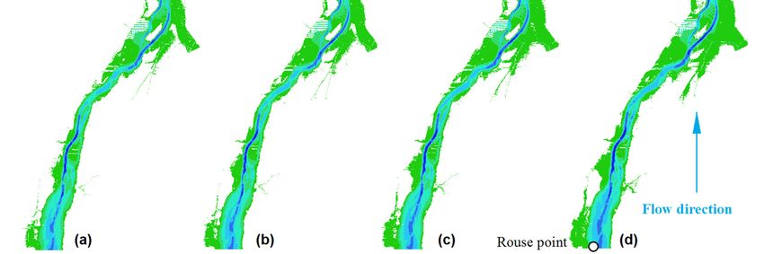
Water2018,
Water 2018,10,
10,272
x FOR PEER REVIEW 44 of
of19
22
was used to solve the shallow water equations. A discussion of how the uncertainty results can be
coefficient and topography,
used is provided at the end.for four different flow rates. An uncertainty assessment was conducted
for a 46 km long reach of the Richelieu River, Canada. The finite-element 2D hydraulic model, H2D2,
was used to solve the shallow water equations. A discussion of how the uncertainty results can be
2. Methods
used is provided at the end.
The uncertainty analysis method proposed involved the following steps: (i) define the
2. Methods distribution for each of the input variables: X (flow rate), X (Manning’s coefficient)
probability
and X (topography); (ii) generate sampled inputs for the identified variables by using PEM; (iii) run
The uncertainty
the hydraulic model analysis
based onmethod proposed
these input involved
parameters the following
(recalculate steps: for
the model (i) define the probability
each sampled input);
distribution for each of the input variables: X (flow rate),
and (iv) quantify the uncertainty of the model1 outputs by computing X 2 (Manning’s coefficient) and X3
the mean and standard
(topography);
deviation of the (ii)water
generate sampled
depths (Table inputs
1). for the identified variables by using PEM; (iii) run the
hydraulic model based on these input parameters (recalculate the model for each sampled input);
and (iv)
Table quantify
1. General the uncertainty
procedure of theanalysis
for uncertainty model based
outputs by computing
on point the mean
estimate method (PEM)and standard deviation
simulations.
of the water depths (Table 1).
Table 1.Preprocessing Processing
General procedure for uncertainty analysis Postprocessing
based on point estimate method (PEM) simulations.
Preprocessing Processing Postprocessing
PEM approach sampling H2D2 model Propagation of uncertainty
PEM approach sampling H2D2 model Propagation of uncertainty
Parameter sampling Inundation modelling Result analysis
Uncertainty Analysis
2.1. Study
2.1. Study Area
Area
The source
The source ofof the
the Richelieu
Richelieu River
River is
is Lake
Lake Champlain
Champlain in in the
the USA
USA and
and itit empties
empties northward
northward intointo
the St.
the St. Lawrence
Lawrence River,
River,Canada.
Canada. The
The discharge
discharge at at which
which Lake
Lake Champlain
Champlain drainsdrains atat increased
increased rates
rates is
is
controlled mainly by an area of rocky shoals located at St-Jean-sur-Richelieu,
controlled mainly by an area of rocky shoals located at St-Jean-sur-Richelieu, about 36 km downstream about 36 km
downstream
(Figure (Figure 1). Ainconstriction
1). A constriction the Richelieuin the Richelieu
regulates the regulates
outflow from the outflow from Lakeand
Lake Champlain Champlain
dictates
andupstream
the dictates water
the upstream water level
level variations. variations.
The flow The flow
contributions fromcontributions
tributaries were from tributaries
ignored duringwerethe
ignored during
calibration thebecause
process calibration process
of the because
significant of thecapacity
storage significant storage
of Lake capacity ofwhich
Champlain, Lake Champlain,
contributes
which
to morecontributes
than 95% oftothe more than 95%
Richelieu of the
River’s Richelieu
flow into theRiver’s flow into
St. Lawrence the[63].
River St. Lawrence
The model River [63].
covered
The model covered a 46 km long reach of the Richelieu River from Rouses
a 46 km long reach of the Richelieu River from Rouses Point on the US–Canada border to the FryersPoint on the US–Canada
borderDam,
Island to theapproximately
Fryers Island10 Dam, approximately
km downstream 10 km
of the downstream
municipality of the municipality of
of St-Jean-sur-Richelieu St-Jean-
(Figure 1).
Asur-Richelieu
longitudinal (Figure 1). A longitudinal
profile developed from theprofile
LiDARdeveloped from the LiDAR
data was performed data was performed for
for the Saint-Jean-sur-Richelieu
the Saint-Jean-sur-Richelieu
shoal area (Figure 2). shoal area (Figure 2).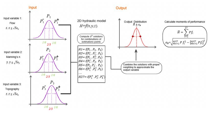
Water 2018, 10, 272                                                                                                5 of 19
Water 2018, 10, x FOR PEER REVIEW                                                                                   5 of 22

Water 2018, 10, x FOR PEER REVIEW                                                                             5 of 22

      Figure 1.
      Figure   1. Location
                  Location of
                           of the
                               the study
                                    studyarea
                                          areawithin
                                              withinthe
                                                     theRichelieu
                                                         RichelieuRiver
                                                                    Riverwatershed
                                                                          watershedtogether
                                                                                     togetherwith
                                                                                               withthethe
                                                                                                        shoal at
                                                                                                          shoal
      Figure 1. Location of the study area within the Richelieu River watershed together with the shoal at
      St-Jean-sur-Richelieu.
      at St-Jean-sur-Richelieu.
      St-Jean-sur-Richelieu.

           Figure
           Figure2.2.Longitudinal
                      Longitudinalprofile
                                   profilefrom LiDAR
                                            from
                                            from     data
                                                 LiDAR
                                                 LiDAR    forfor
                                                       data
                                                       data   thethe
                                                             for  Saint-Jean-Sur-Richelieu
                                                                 the                       shoal
                                                                     Saint-Jean-Sur-Richelieu
                                                                     Saint-Jean-Sur-Richelieu    area.area.
                                                                                               shoal
                                                                                              shoal   area.

2.2. Hydraulic
2.2. Hydraulic Model
                  Modelofof
                         ofthe
                            theRichelieu
                                 RichelieuRiver
                                              River
2.2. Hydraulic Model        the Richelieu    River
      The
      The simulations
          simulations    are based    onona on
                                            atwo-dimensional    finite element   hydraulic   model  of the Richelieu
     The   simulationsare    arebased
                                  based         two-dimensional
                                                  a two-dimensionalfinite  element
                                                                          finite    hydraulic
                                                                                  element       model
                                                                                             hydraulic   ofmodel
                                                                                                            the Richelieu
                                                                                                                   of the
River
River  using
       using  the
               the  H2D2
                     H2D2   software
                             software  [64].
                                         [64].  H2D2
                                                 H2D2 solves
                                                        solvesthe 2D
                                                                the   depth-averaged
                                                                     2D   depth-averaged  shallow-water
                                                                                              shallow-waterequations
                                                                                                               equations
Richelieu River using the H2D2 software [64]. H2D2 solves the 2D depth-averaged shallow-water
(SWE) based on the conservative form of mass Equation (2) and the two equations of momentum
(SWE) based
equations   (SWE)on the   conservative
                      based    on the        form of mass
                                        conservative         Equation     (2) and the (2)
                                                                                        twoandequations
                                                                                                      twoofequations
                                                                                                             momentum
conservation    (3) and (4) under    steady-state    flowform   of mass
                                                          conditions   withEquation
                                                                              special treatment  thedrying–wetting
                                                                                                 of                     of
conservation
momentum         (3) and  (4) under    steady-state    flow  conditions    with  special  treatment
              conservation (3) and (4) under steady-state flow conditions with special treatment of  of  drying–wetting
areas.
areas.
drying–wetting      areas [65].
                                                          +      = 0,                                             (2)
                                                             +      =
                                                                     0,2                                              (2)
                                                                       ∂ h ∂2 h
                                                    ∂qy
                                  ∂h       ∂qx
                                      +          +       + ( γ + δ)       2
                                                                            +     2
                                                                                       =  0                            (2)
                            +     ∂t      +∂x c    −∂y (Hτ ) + ∂xHτ ∂y− τ − τ ) − f q = 0,                        (3)
                             +              +c       −       (Hτ ) +          Hτ − τ − τ ) − f q = 0,                  (3)
Water 2018, 10, 272 6 of 19
q q
∂qx ∂ qx qx ∂ x y ∂h 1 ∂ ∂
+ c2 Hτxy − τbx + τsx − fc qy = 0 (3)
+ + − × (Hτxx ) +
∂t ∂x H ∂y H ∂x ρ ∂x ∂y
∂ qy qx
∂qy q q
∂ y y 2 ∂h 1 ∂ ∂ b s
+ + +c − × Hτyx + Hτyy − τy + τy + fc qx = 0 (4)
∂t ∂x H ∂y H ∂y ρ ∂x ∂y
Water 2018, 10, x FOR PEER REVIEW 6 of 22
where qx and qy are the flow rates in x and y direction (m2 /s), h is the water level (m), H is the depth
of water, c is wave velocity + (m/s), ρ is + the
c density,
− u(u, v+) areHτ
Hτ the components
− τ − τ ) + f of q the
= 0,of velocity (4) vector
(m/s), γ Lapidus coefficient, δ hydraulic conductivity (set to 0 in wet areas and to 1 in dry areas), fc
where qforce,and q τ are the flow rates in x and y direction 2 (m b⁄s), h isb the water level (m), H is the
is the Coriolis ij is the Reynolds stresses (m/s m), τx and τy are the bottom frictions in the x
depth of water, c2 is wave velocity (m ⁄s) , r is the water density, ρ is the density, u(u, v) are the
and y directions (kg/s m), τsx and τsy are the surface frictions in the x and y directions (kg/s2 m), and
components of the of velocity vector (m⁄s) , f is the Coriolis force, τ is the Reynolds stresses
x(x, y) are
(m⁄sthe m)components
, τ and τ areof thecoordinate
bottom frictionsorientation
in the x of X(ymdirections
and ). The continuous
(kg⁄s m), τ fields
and τ h, areuthe
and v are
discretized over a unstructured mesh of finite element triangles of six nodes,
surface frictions in the x and y directions (kg⁄s . m), and x(x, y) are the components of coordinate referred to as T6L.
The H2D2 model
orientation of X(m).is The
basedmodelondoesthe not
assumptions
take into account of incompressibility, hydrostatic
the influence of the wind pressure, and
and the Coriolis
force. The continuous
stable riverbed. fields h, u discretization
The finite-element and v are discretized has beenover adetailed
structuredbymesh of finite
[66,67]. Theelement
H2D2 model
triangles
calculates the flowof sixvelocity,
nodes, referred
dischargeto as and
T6L. water levels in a 2D domain using an implicit time scheme
The H2D2 model is based on the assumptions of incompressibility, hydrostatic pressure, and
and direct Newton Raphson steps. In doing so, it also takes into account the wetting and drying of
stable riverbed. The finite-element discretization has been detailed by [65,66]. The H2D2 model
the rivercalculates
banks, based
the flowon the water
velocity, flowand
discharge andwater
levellevels
[65].inThea 2Dfinite
domain element
using anmesh stores
implicit timeall of the input
scheme
variables
and needed for theRaphson
direct Newton resolution steps. ofInSt-Venant
doing so, itequations, as well
also takes into as the
account resulting
the wetting andvariables
drying of for the
2D flowthesimulation
river banks,(water
based on level and velocities).
the water flow and level The advantage
[67]. of using
The finite element thisstores
mesh software is its
all of the simplicity
input
in termsvariables
of dataneeded for the resolution
requirements and most of St-Venant
particularly equations, as well as the
the possibility resulting variables
of modifying for the
the river geometry,
2D flow simulation (water level and velocities). The advantage of using this software is its simplicity
qualities that have been demonstrated in several flood inundation studies [68,69].
in terms of data requirements and most particularly the possibility of modifying the river geometry,
First, H2D2 was applied in the Richelieu River watershed located about 20 km east of Montreal,
qualities that have been demonstrated in several flood inundation studies [68–70].
Canada (FigureFirst, 1).
H2D2 Thewasmodel
applied had been
in the pre-calibrated
Richelieu River watershedby Environment
located aboutCanada
20 km east with the high water
of Montreal,
event ofCanada
6 May(Figure
2011, 1).
under steady-state
The model had beenflow conditions
pre-calibrated by without
Environment wind forcing
Canada with[70]. The water
the high flow during
event
the survey of 6at
was Mayan 2011, under steady-state
approximate rate of 1550flow m 3 /s at the
conditions without
Fryers wind forcing
Rapids [71]. Thestation.
gauging flow during
Calibration
the survey was at an approximate rate of 1550 m ⁄s at the Fryers Rapids
was carried out by adjusting the Manning’s coefficient. There was a difference between simulated and gauging station. Calibration
was carried out by adjusting the Manning’s coefficient. There was a difference between simulated
measured water levels at Saint-Jean-sur-Richelieu of 1cm. The results for the calibration for this high
and measured water levels at Saint-Jean-sur-Richelieu of 1cm. The results for the calibration for this
event on 6 May
high event2011
on 6 are
Maypresented in Figure
2011 are presented 3.
in Figure 3.
Figure 3. Profile
Figure of of
3. Profile measured
measured and simulated
and simulated levels
levels for for 6 May
6 May 2011.2011.
The Richelieu River model developed for this analysis covered a 46 km long reach of the
TheRichelieu
Richelieu
RiverRiver
frommodel
Rousesdeveloped
Point on the for this analysis
US–Canada bordercovered a 46Island
to the Fryers km long
Dam,reach of the Richelieu
approximately
River from
10 km downstream of the municipality of St-Jean-sur-Richelieu. The model domain was discretized 10 km
Rouses Point on the US–Canada border to the Fryers Island Dam, approximately
downstream of the municipality
over a structured mesh of 47,643of finite
St-Jean-sur-Richelieu. The model
elements and 97,261 nodes, with a domain was
regular size of discretized
25 m. The over
model input
a unstructured meshconsisted
of 47,643offinite
DEM,elements
with coordinates x, ynodes,
and 97,261 and z with
interpolated
a regularandsize
projected to The
of 25 m. the model
hydraulic mesh, and the boundary conditions and Manning’s coefficient as the calibration parameters.
input consisted of DEM, with coordinates x, y and z interpolated and projected to the hydraulic mesh,
The influence of the wind forces and the Coriolis effect were not considered. This is because there
and thewas
boundary conditions and Manning’s coefficient as the calibration parameters. The influence
insufficient information to describe the uncertainty in the wind data available for the Richelieu
of the wind forces and the
River. The resulting Coriolis
water depthseffect were notby
were calculated considered. This is
subtracting water because
surface there from
elevations was river
insufficient
information to describe
bed elevations. Thethe uncertainty
model in evaluate
was used to the wind thedata available
water levels andfor theinRichelieu
flow River.
the Richelieu The
River. resulting
The
water level
water depths wereinformation
calculatedcouldbythen be utilized by
subtracting othersurface
water studies relating to the from
elevations impactriver
of water
bedlevels
elevations.
in thewas
The model river. In all
used toofevaluate
these applications
the water no levels
quantification
and flow of uncertainty in the model
in the Richelieu River.outputs was level
The water
made. The model took approximately one hour to provide a steady-state solution on a computer with
information could then be utilized by other studies relating to the impact of water levels in the river.
a core i7 processor of 3.6 GHz and 16 Gigabytes of RAM (Random access memory).Water 2018, 10, 272 7 of 19
In all of these applications no quantification of uncertainty in the model outputs was made. The model
took approximately one hour to provide a steady-state solution on a computer with a core i7 processor
of 3.6 GHz and 16 Gigabytes of RAM (Random access memory).
The topography data for the model was determined using a DEM with a cell size of 1 × 1 m2
and an accuracy of ±0.3 m derived from LiDAR datasets obtained in 2008, 2010, and 2011, provided
by Environment Canada (EC). Based on the various classes of point from the data sources, EC used
only the ground class, which represents 85% of the LiDAR points surveyed. The other classes, such as
the building and vegetation, were not used in the DEM. A set of orthophotos from the 2009 database
for the administrative region of Montérégie, Quebec was used to validate the limits of the water
courses. The elevations of the points below the water surface came from bathymetry data. Bathymetric
information describes the geometry of a river. The bathymetry of the riverbed was taken from the
Canadian Hydrographic Service (low river) and bathymetric transects were provided by Parks Canada
(mid river). To import topobathymetry into the model, the individual soundings were interpolated
onto the finite element grid nodes. The interpolation of each individual sounding reduces the amount
of uncertainty in the bathymetry in the model. Uncertainties in the bathymetric data were not explicitly
dealt with in this study. The range of calibrated Manning’s coefficients between of 0.02–0.036 was
used as the mean value of the random field over the study area. The substratum upstream consists
of fine sand and silt. The substrate is much coarser with some boulders, approaching the shoal
in Saint-Jean-sur-Richelieu.
The upstream boundary condition of the model is the flow rate at Rouses Point and stage
conditions used at the downstream limit of the model near the Fryers Rapids station (EC 02OJ007).
The water level was estimated using the established stage–discharge relationships. Q and H are,
respectively, the discharge (m3 /s) and water level (m)
H = Q/303.37(1/1.727) + 25.52 (5)
2.3. Point Estimate Method
Knowledge of the mean and the standard deviation of each input variable at each of the model’s
grid cells is necessary to compute the combined uncertainty of the outputs using the PEM. The method
estimates the mean and standard deviation of a performance function using statistical moments of the
random input variables. Originally proposed by Rosenblueth [71], the method has been improved in
the past decade [72,73]. The objective is to evaluate the model at a discrete set of points in the uncertain
parameter space and to combine uncertainties of the random variables with proper weighting in order
to calculate the mean and standard deviation of the output, which is the water depth in this case. These
outputs provide useful information for researchers and managers, but in the absence of uncertainty
information, the mean values alone do not show the expected range of possible water depth values.
The standard PEM considers a set of random variables Xi (X1 , X2 . . . , Xn ) with a probability
distribution function fXi (x), and a performance function Y, obtained from the deterministic relationship
of X (Y = g(Xi )) to represent the output variable Yi. In this application, the considered independent
random variables include the flow rate as the upstream boundary condition, Manning’s coefficient,
and topography. In this case, the performance function is the water depth, g(x). The input variables
are stochastic, i.e., they can be described in terms of their mean and variance. The PEM method is
used to approximate the mean, variance, and/or higher moments of the outputs. The accuracy of
the prediction of the uncertainty in the model outputs depends largely on the ability to estimate the
uncertainty in the inputs.
The statistical moments of the model output can be calculated in terms of the respective moments
of the input as follows: Z
uXm = (x − µX )m fX (x)dx, (6)
where uxm is moment of order m and µX is the first moment of fX (x). The integrals given in Equation (4)
are solved by applying the approximate integration with PEM. The continuous random variable X isWater 2018, 10, 272 8 of 19
replaced by a discrete random variable with a probability mass function (pmf) of the same moment
order m as fx (x). The pmf pX (x) is transformed using g(X) to obtain another discrete function with
pmf pY (y). In the continuous case, pY (y) is used to calculate the moments of Y. In the case of a 1D
integral, the mth central moment of fX (x), µXm , is obtained as follows:
Z
uXm = (x − µX )m fX (x)dx = ∑(x − uX )m pX (x), (7)
The optimal coordinates are those at which the integral and the corresponding weights are selected
by the Gaussian quadrature procedures. In fact, the PEM can be considered as an application of the
Gaussian quadrature procedures [74]. Table 2 shows the coordinates along the abscissa and weights
for the three first quadrature formulas based on the normal distribution as the weight function.
√
Table 2. Coordinates and weights for the standard normal distribution (x = 2 σz).
Number of Node (N) Coordinate xi Weights Ai
0 0 1
1 − 1 1
√ 1,1 √ 2, 2
1 2 1
2 − 3, 0, 3 6 3, 6
,
For a case in which the performance function involves n independent random variables assumed
to be approximately Gaussian, Rosenblueth suggested that x can be estimated at more than two points.
The three-point method applied herein considers a central point at x = µx and two points x+ and x−
symmetrically distributed around the mean. Designating the weight of the central point as P and of
the other two points as P_ and P+, the respective weights can be written as:
2P+ + P = 1, (8)
2P+ (x+ − µx )2 = σ2X , (9)
2P+ (x+ − µx )4 = 3σ4X , (10)
The solutions of these equations gives the following results:
2 1
P= ; P+ = P− = , (11)
3 6
√
x± = µX ± 3σX , (12)
In most cases, the calculations are made at two points and the expected value of the k-th power of
the probability distribution of Y is determined by:
m m m
E[Ym ] = P− y− + P yµ + P+ y+ , (13)
where Y is a deterministic function of X = g(X); E[Ym ] is the expected value of Y to the power m;
y+ is the value of Y at the upper point x+ , which is greater than the mean µx ; y− is the value of Y at
the lower point x− , which is less than the mean µx ; ym is the value of Y at the mean µx . If m is large,
the method requires a considerable computational effort, as is the case with 2D SWE models.
To assess the uncertainty propagation, the performance of the model is evaluated through (n + 1)p
simulations, where: p is the number of uncertain variables and n is number
√ of nodes. Each simulation
corresponds to the perturbation of a given random variable with a ± 3 standard deviation about its
mean value. The point estimate method needed only 27 calculations of the H2D2 model for each flow
case. The PEM method is relatively simple in formulation when compared to other uncertainty analysis
methods, such as the Monte Carlo Method. The disadvantage of Monte Carlo analysis is that it can beWater 2018, 10, 272 9 of 19
computationally demanding. This can be an issue for complex models that require a significant amount
of time to compute. Figure 4 shows the procedure applied to estimate the statistical moments of the
model output for three input variables. For the purpose of numerical computation, the random fields
of the uncertain parameters are represented in terms of uncorrelated random variables. The H2D2
model of2018,
Water the10,Richelieu
x FOR PEER River
REVIEW calculates values for Equation (13) at all the nodes within 9 of 22the model
domain. PEM simulations were conducted by using three variables with the proper weighting (Table 3).
uncorrelated random variables. The H2D2 model of the Richelieu River calculates values for Equation
The sum of the all weights is equal to 1. The disadvantage of PEM is that it loses precision as the
(13) at all the nodes within the model domain. PEM simulations were conducted by using three
nonlinearity
variables of thethemodel
with properincreases
weightingand if the
(Table 3). moments
The sum ofhigher
the all than theissecond
weights equal to moment
1. The are to be
obtained, and theoffast
disadvantage PEMgrowing
is that itofloses
the number
precision of
as calculations
the nonlinearityneeded
of the if the number
model increasesof random
and if the variables
increases,
moments which
higher increases the complexity
than the second moment are of theobtained,
to be analyses andand thegrowing
the fast computation time [73].
of the number of This is
calculations needed if the number of random variables increases, which increases
especially the case if the input parameters are correlated, requiring the computation of covariance for the complexity of
each the
pairanalyses and theand
of variables computation
inclusiontime [74].
of the This is especially
co-variances in thetheuncertainty
case if the input parameters
calculations are
Therefore, PEM
correlated, requiring the computation of covariance for each pair of variables and inclusion of the co-
gave reliable and accurate results with the third lowest moments. It is relatively easy to run with the
variances in the uncertainty calculations Therefore, PEM gave reliable and accurate results with the
bulk third
of the effortmoments.
lowest requiredIt to utilize the
is relatively method.
easy The the
to run with disadvantage of the
bulk of the effort PEM method,
required to utilize is
thethat it does
not provide
method. The disadvantage of the PEM method, is that it does not provide a measure of the influenceit is not an
a measure of the influence of each random variable to the overall variance, so
adequate
of eachmethod
randomto filter the
variable most
to the relevant
overall random
variance, so it is variables. Also,method
not an adequate the PEM method
to filter does not take
the most
into account the distribution of the input parameters. It relies only on the mean and of
relevant random variables. Also, the PEM method does not take into account the distribution thethevariance to
input parameters. It relies only on the mean and the variance to describe the parameter. Some of the
describe the parameter. Some of the shortcomings of the method arise from the reality that the PEM
shortcomings of the method arise from the reality that the PEM method is an approximate uncertainty
method is an approximate uncertainty analysis method.
analysis method.
Figure
Figure 4. Basic
4. Basic principlesof
principles of the
the point
pointestimate method
estimate for estimation
method of the statistical
for estimation moments of
of the statistical the
moments of the
output parameter based on three independent normal random input variables (H , σ ) are the mean
output parameter based on three independent normal random input variables (H , σH ) are the mean
and the standard deviation of water depth.
and the standard deviation of water depth.
Table 3. The conditions for uncertainty analysis of topography, Manning’s and flow rate using the
Table 3. The
PEM conditions for uncertainty analysis of topography, Manning’s and flow rate using the
method.
PEM method. Case Topography Manning’s Flow Rate Weight
1
Case
Case H1 Topography
Min Manning’s Min Flow Rate
Min Weight
216
Case H1 Min Min Min 1
2 216
2
Case
Case H2H2 Min
Min Min Min Mean Mean
108 108
1
Case H3 Min Min Max 1 216
Case H3 Min Min Max 2
Case H4 Min Mean Min216 108
Case H5H4 Min 2 4
Case Min MeanMean Min Mean 54
Case H6 Min Mean Max108 2
4 108
1
Case
Case H7H5 Min
Min MeanMax Mean Min
54 216Water 2018, 10, 272 10 of 19
Table 3. Cont.
Case Topography Manning’s Flow Rate Weight
Case H8 Min Max Mean 2
108
Case H9 Min Max Max 1
216
Case H10 Mean Min Min 2
108
Case H11 Mean Min Mean 4
54
Case H12 Mean Min Max 2
108
Case H13 Mean Mean Min 4
54
Case H14 Mean Mean Mean 8
27
Case H15 Mean Mean Max 4
54
Case H16 Mean Max Min 2
108
Case H17 Mean Max Mean 4
54
Case H18 Mean Max Max 2
108
Case H19 Max Min Min 1
216
Case H20 Max Min Mean 2
108
Case H21 Max Min Max 1
216
Case H22 Max Mean Min 2
108
Case H23 Max Mean Mean 4
54
Case H24 Max Mean Max 2
108
Case H25 Max Max Min 1
216
Case H26 Max Max Mean 2
108
Case H27 Max Max Max 1
216
3. Quantification of Uncertainty
3.1. Flow Rate
The reference flow rates for the hydraulic model were determined by analyzing the frequency of
daily recordings at the Fryers Rapids station (between 1972 to 2011). To fully investigate the uncertainty
in potential flood events, four flow rates were imposed to constrain the model: 759, 824, 936, 1113 m3 /s.
These values are related to four return periods: 1.25, 1.4, 2, and 5 years used by Quebec’s public safety
ministry. The hydrologic uncertainty was determined with the standard error of the design flow rate,
assuming that its distribution
√ is normal [20] (Table 4). The perturbed discharge Qt is calculated as the
mean discharge Qbase ± 3 standard deviation.
√
Qt = Qbase ± 3σ (14)
The set of three values for each flow rate Equation (14) was used to obtain the perturbed flow rate
considered as an upstream boundary condition for assessment of the performance function (Table 4).
Table 4. Flow rates used to evaluate the performance function with the point estimate method.
√ √
µ σ xi − 3σ xi + 3σ
759 39.4 690.75 827.24
824 36 761.64 886.35
936 33.7 877.62 994.37
1113 39.4 1044.75 1181.24
3.2. Manning’s n Coefficient
The basic roughness parameters were derived from tabulated values [75] and further modified
during the calibration the model. The Manning’s n coefficient is assumed to be normally distributed
about the mean values calibrated during the calibration process of the model [26–28] and not through
field measurements or observations. The mean n values vary spatially across the domain within theWater 2018, 10, 272 11 of 19
range of 0.02 to 0.036, inferred from substrate samples, and the standard deviation was calculated
based on the 3σ rule as 0.0026 (s/m1/3 ) [76].
σ = (Mmax − Mmin )/6, (15)
The uncertainty in the Manning’s n is likely smaller. The reason for this is the calibration process,
which makes use of river water levels to indirectly determine the appropriate Manning’s n value.
Still, the calibration process is not exact and even though these parameters are optimally determined
through calibration, they could still be incorrect or have some degree of uncertainty in them. There are
alternative parametrization methods that perform almost as well as the optimal Manning’s n values.
There is also the possibility that the Manning’s n parameters may be compensating for errors in other
aspects of the model, such as channel bathymetry.
The three random fields generated by the input of the Manning’s coefficient in the H2D2, used
to evaluate the model’s performance,√ are provided Figure 5. It involves changing the Manning’s
coefficient along the river by the 3 error. For example, this change happens in the area with sills or
where the bathymetry suggested a coarser substrate. An increase in the coefficient (upper scenario)
yields a lower flow and a higher water level. However, the decrease in the coefficient (lower scenario)
includes shallow water depth, faster velocities, and supercritical flows.
Water 2018, 10, x FOR PEER REVIEW 12 of 22
Figure 5. Three images of the random field of Manning’s coefficient: (a) lower scenario (μ − √3σ); (b) √
Figure 5. Three images
nominal scenarioof(μ);
the random
and (c) higherfield of Manning’s
scenario (μ
+ √3σ). coefficient: (a) lower scenario (µ − 3σ);
√
(b) nominal scenario (µ); and (c) higher scenario µ + 3σ .
3.3. Topography
To investigate the effect of topography uncertainty on model predictions, a standard deviation
related to each grid cell was generated by kriging the DEM used as the mean value. As was the case
in the evaluation of the Manning’s coefficient, it was hypothesized that the errors related to the
estimation of topography follow a normal distribution and are independent [39–41]. Kriging was
performed by applying a locally adaptive exponential variogram to the entire study area with a sill
value of 0.8 m and nugget effect of 0.03 m (0.18 = 0.03). The sill implies the variance of the data.Water 2018, 10, 272 12 of 19
3.3. Topography
To investigate the effect of topography uncertainty on model predictions, a standard deviation
related to each grid cell was generated by kriging the DEM used as the mean value. As was the case in
the evaluation of the Manning’s coefficient, it was hypothesized that the errors related to the estimation
of topography follow a normal distribution and are independent [39–41]. Kriging was performed by
applying a locally adaptive exponential variogram to the entire study area with a sill value of 0.8 m2
and nugget effect of 0.03 m2 0.182 = 0.03 . The sill implies the variance of the data. The nugget
could represent the measurement error or some variation at small scale. The error represents the
vertical accuracy DEM (±15 cm), and the vertical error specific to the airborne positioning system
(3 cm). The kriging variances were then transformed into standard deviation (i.e., the square root
of estimation variance). Figure 6a shows the highest standard deviation with a maximum value
of 0.21 m. These changes are incorporated in the steady-state hydraulic model. To quantify the
topography’s uncertainty, the kriged standard deviation was added to and √ subtracted from the
Water 2018, 10, x FOR PEER REVIEW 13 of 22
DEM (mean topography) to obtain the upper and lower confidence levels (± 3 standard deviation).
With this change, With
deviation). the topography
this change, thebehaves as a behaves
topography flexibleasbody because
a flexible body it will move
because it will up or up
move downor from
a normaldown
distribution and therefore
from a normal lead
distribution andtotherefore
the change
lead in the change
to the simulated
in thewater surface
simulated elevations
water surface from
elevations from the hydraulic
the hydraulic modelling. The random
fieldstopography
generatedfields generated by perturbing the
√mean modelling.
topography
The random
by the √3
topography
error are given in Figures 6b–d.
by perturbing
With these
the mean topography
perturbations, the
by the 3 error are given in Figure 6b–d. With these perturbations, the topography was moved up
topography was moved up and down from the mean values, which resulted in a change of the
and down from the mean values, which resulted in a change of the simulated water surfaces (without
simulated water surfaces (without varying the flow rate and Manning’s coefficient in the hydraulic
varying model).
the flow rate and Manning’s coefficient in the hydraulic model).
Figure 6.Figure 6. Topography (a) standard deviation, and representations of the random topography fields:
Topography (a) standard deviation, and representations of the random topography fields:
(b) lower topography scenario; (c) mean topography scenario; and (d) upper topography scenario.
(b) lower topography scenario; (c) mean topography scenario; and (d) upper topography scenario.
4. Uncertainty in the Model Output
Having defined the individual uncertainty in the three input variables, PEM simulations were
performed in combination with H2D2 to assess the uncertainty which is propagated into the output
values. For a given flow rate, the hydraulic model was only run 27 times, in agreement with the 3 × 3
× 3 combinations associated with the μ and μ ± √3σ random fields of the three input variables. The
mean and the standard deviation of the water depth for each grid cell were calculated with EquationWater 2018, 10, 272 13 of 19
4. Uncertainty in the Model Output
Having defined the individual uncertainty in the three input variables, PEM simulations were
performed in combination with H2D2 to assess the uncertainty which is propagated into the output
values. For a given flow rate, the hydraulic model was √ only run 27 times, in agreement with the
3 × 3 × 3 combinations associated with the µ and µ ± 3σ random fields of the three input variables.
The mean and the standard deviation of the water depth for each grid cell were calculated with
Equation (11). Therefore, to fully investigate the uncertainty distributions, 108 model runs (4 × 27)
were sufficient to obtain the expected mean and standard deviation of the water depth for the four
reference flow rates 759, 824, 936, 1113 m3 /s. The H2D2 model was prepared to explore the transfer of
variability from the Manning’s coefficient, flow rate and topography to water depth under steady-state
application, without
Water 2018, 10, non-linear
x FOR PEER REVIEW perturbations. Each run of the H2D2 model had an average 14 of 22 time
duration of 1 h, which makes flood uncertainty analysis with Monte Carlo unfeasible from a practical
pointduration
of viewofin1 engineering.
h, which makes flood
Still, anuncertainty
approximateanalysis with Monte
uncertainty Carlo
analysis unfeasible
can from a with
be performed practical
the help
point
of the of view
point estimate in engineering.
method. The Still, an approximate
mathematical uncertainty
operations analysis
defined can be performed
in Equation (13) werewith the
performed
help of the point estimate method. The mathematical operations defined in Equation (13) were
within the GIS using the simulated layers with H2D2. The resulting spatial distributions of the mean
performed within the GIS using the simulated layers with H2D2. The resulting spatial distributions
and the standard deviation of the outputs are shown in Figures 7 and 8, respectively, which were
of the mean and the standard deviation of the outputs are shown in Figures 7 and 8, respectively,
obtained by implementing the point estimate calculations within the GIS software. The expected
which were obtained by implementing the point estimate calculations within the GIS software. The
value or mean
expected valueof or
themean
water depths
of the waterwas determined
depths by running
was determined the model
by running with
the model thethe
with mean
meaninput
parameter values.
input parameter values.
Figure 7. Mean values of the water depths predicted with the point estimate method for four flow
Figure 7. Mean values of the water depths predicted with the point estimate method for four flow
rates: (a) 759 m ⁄s ; (b) 824 m ⁄s ; (c) 936 m ⁄s ; and (d) 1113 m ⁄s.
rates: (a) 759 m3 /s ; (b) 824 m3 /s ; (c) 936 m3 /s ; and (d) 1113 m3 /s.Water 2018, 10, 272 14 of 19
Water 2018, 10, x FOR PEER REVIEW 15 of 22
Figure
Figure88.. Standard
Standarddeviations
deviationsof water depth
of water predicted
depth with the
predicted point
with theestimate method for
point estimate four flow
method rates:flow
for four
( ) 759 m ⁄s ; ( ) 8243 m ⁄s ; ( ) 936 3m ⁄ s ; and ( ) 1113
3 m ⁄s .
rates: (a) 759 m /s ; (b) 824 m /s ; (c) 936 m /s ; and (d) 1113 m /s. 3
It can be observed in Figures 7 and 8 that the expected water depths were below 12.06 m deep,
It can be observed in Figures 7 and 8 that the expected water depths were below 12.06 m deep,
whereas the overall standard deviations were less than 27 cm for the four flow rates. The highest
whereas the overall standard deviations were less than 27 cm for the four flow rates. The highest water
water depths were located downstream of Saint-Jean-sur-Richelieu. At Saint-Jean-sur-Richelieu, the
depths were located
river becomes narrower downstream
and the bottom of Saint-Jean-sur-Richelieu.
rises to the head of the rapids At Saint-Jean-sur-Richelieu,
near the shoal. In this reachthe river
becomes narrower and the bottom rises to the head of the rapids
the slope of the river is quite steep where the riverbed is composed of a coarser near the shoal.Below
substrate. In this
thereach the
slope of the river is quite steep where the riverbed is composed of a coarser substrate.
shoal, the slope of the river becomes flatter until the downstream limit is reached. The upstream reach, Below the
shoal, the slope
from Rouses Pointoftothe river becomes flatteris until
Saint-Jean-sur-Richelieu, the downstream
characterized limit depths.
by lower water is reached. The isupstream
The river
wide and
reach, fromtheRouses
impediment
Point to
to flow is not great, it is a lake-like
Saint-Jean-sur-Richelieu, section of the
is characterized byriver with
lower a very
water minorThe river
depths.
gradient.
is wide andThisthe
region can be considered
impediment to flowasisannot
extension
great, ofit Lake Champlain.
is a lake-like The spatial
section of thedistribution
river with a very
of the standard
minor gradient.deviations
This regionshowscanhigher standard deviations
be considered in the upstream
as an extension of Lake close to the shoalThe
Champlain. in spatial
Saint-Jean-sur-Richelieu, and lower standard deviations in the far upstream (Figures 8). The increase
distribution of the standard deviations shows higher standard deviations in the upstream close to
in uncertainty in water depth is directly proportional to the increase in uncertainty in these model
the shoal in Saint-Jean-sur-Richelieu, and lower standard deviations in the far upstream (Figure 8).
parameters. This finding is expected due to the equation used for calculating the uncertainty,
The increase in uncertainty in water depth is directly proportional to the increase in uncertainty in these
Equation (12). Water depth upstream of Saint Jean is therefore influenced almost entirely by the shoal.
model parameters.
The lower This finding
standard deviation near is
theexpected due to theis equation
model boundaries probably inused
partfor calculating
due the uncertainty,
to the fact that the
Equation
water level(12). Water depth
is controlled upstream
at these locationsofdirectly
Saint Jean
at theisdownstream
therefore influenced almost
boundary and entirely
indirectly byby
thethe shoal.
The lower standard deviation near the model boundaries is probably in part due to the fact that the
water level is controlled at these locations directly at the downstream boundary and indirectly by the
influence of the upstream boundary defined by the constant flow rate. It can also be observed thatWater 2018, 10, 272 15 of 19
Water 2018, 10, x FOR PEER REVIEW 16 of 22
an increase of the flow rate from 759 m3 /s (Figure 8a) to 1113 m3 /s (Figure 8d) slightly decreases the
influence of the upstream boundary defined by the constant flow rate. It can also be observed that an
standard deviations of the water depth3 values. This can be explained by the hydraulic model for the
increase of the flow rate from 759 m /s (Figure 8a) to 1113 m3/s (Figure 8d) slightly decreases the
Richelieu River, which was solely calibrated for the high-water event of 6 May 2011, using a flow rate
standard deviations of the water depth values. This can be explained by the hydraulic model for the
1550 m3 /s.
of Richelieu River, which was solely calibrated for the high-water event of 6 May 2011, using a flow rate
of These
1550 mfindings
3/s. indicate that the water depths upstream of Saint-Jean-sur-Richelieu are therefore
highly These
sensitive to the
findings shoal’sthat
indicate topography at Saint-Jean-sur-Richelieu.
the water depths The upstream
upstream of Saint-Jean-sur-Richelieu arewater slope
therefore
therefore
highly sensitive to the shoal’s topography at Saint-Jean-sur-Richelieu. The upstream water slope of
remains a function of the streambed roughness, since the rivers primary level and rate
discharge
therefore is remains
limited to its capacity
a function at the
of the shoal. From
streambed the point
roughness, of view
since of theprimary
the rivers engineer thatand
level hasrate
to build
of
a model,
discharge theislocation
limited of to these zones at
its capacity with
thehigher variability
shoal. From can of
the point be view
useful oftothemake decisions
engineer such
that has to as
where
buildtoa direct
model,efforts to efficiently
the location improve
of these zones withthe model.
higher The higher
variability can beuncertainty
useful to makelocated at thesuch
decisions reach
as wheremay
upstream to direct efforts to by
be explained efficiently improve
the presence of the model. The higher uncertainty
Saint-Jean-sur-Richelieu located
shoal. at thecontains
The latter reach
upstream
some may be explained
anthropogenic submerged by structures
the presence of the
such Saint-Jean-sur-Richelieu
as steel traps for fishing nets shoal.
and The
milllatter
racescontains
(Figure 9).
At some anthropogenic
low flow rates, thesesubmerged
structures fillstructures
with water suchwithout
as steelcontributing
traps for fishing nets
to the flowand mill races
because the (Figure
velocities
9). At low flow rates, these structures fill with water without contributing
are very low, and probably act as a natural sills at low flow rates. Therefore, they are a significant to the flow because the
velocities are very low, and probably act as a natural sills at low flow
contributing factor to the hydraulic response of this basin. The submerged structures would require rates. Therefore, they are a
significant
relocation contributing
because factorwater
of increased to thedepths
hydraulic response of
and generally this basin.
unsuitable The submerged
conditions structures
for trapping created
would require relocation because of increased water depths and generally
by dredging and structure operations. The important effect of the shoal on low flow regimes was unsuitable conditions forthe
trapping created by dredging and structure operations. The important effect of the shoal on low flow
reason that the hydraulic model for the Richelieu River was calibrated for the high water event of
regimes was the reason that the hydraulic model for the Richelieu River was calibrated for the high
6 May 2011. For this reason, and in order to build an accurate 2D hydraulic model, the topography
water event of 6 May 2011. For this reason, and in order to build an accurate 2D hydraulic model, the
of the model should be carefully considered, especially in the shoal, possibly by acquiring a new
topography of the model should be carefully considered, especially in the shoal, possibly by
river bathymetry.
acquiring a new river bathymetry.
Figure 9. Submerged structures in the Saint-Jean-sur-Richelieu shoal area.
Figure 9. Submerged structures in the Saint-Jean-sur-Richelieu shoal area.
5. Conclusions
5. Conclusions
Water depth uncertainties were quantified as the output of the two-dimensional hydraulic
WaterThe
model. depth uncertainties
uncertainty were quantified
propagated as thevariables
from the input output oftothethetwo-dimensional
model’s output washydraulic model.
calculated
The uncertainty
using the pointpropagated from the
estimate method inputTovariables
(PEM). to thethe
demonstrate model’s output
practical was calculated
applicability of the PEMusing
forthe
point estimateanalyses,
uncertainty method the
(PEM). To demonstrate
hydraulic model H2D2the waspractical
applied applicability of the
over a 46 km long PEM
reach of for
the uncertainty
Richelieu
River, Canada.
analyses, Three random
the hydraulic variables
model H2D2 waswere considered
applied over a 46to be
kmsources of uncertainty:
long reach flow rate,
of the Richelieu River,
Manning’s
Canada. coefficient
Three and topography.
random variables The combined
were considered uncertainty
to be sources was calculated
of uncertainty: flowusing
rate, the PEM
Manning’s
analysis and
coefficient method.
topography. The combined uncertainty was calculated using the PEM analysis method.You can also read