Temperature compensation design and experiment for a giant magnetostrictive actuator
←
→
Page content transcription
If your browser does not render page correctly, please read the page content below

www.nature.com/scientificreports
OPEN Temperature compensation
design and experiment for a giant
magnetostrictive actuator
Zhangrong Zhao1 & Xiaomei Sui2*
Because the performance of giant magnetostrictive materials (GMMs) can vary at different
temperatures, the positioning accuracy of a giant magnetostrictive actuator is affected by heat. In
this work, a new simplified control strategy under compulsory water cooling is proposed to maintain
a constant GMM temperature. Based on this strategy, a coupled turbulent flow field and temperature
field finite element model is created for a GMM smart component. The model is simulated using
COMSOL Multiphysics software version 5.3. Through simulations, the temperature field distribution
of GMM smart components is analysed under different drive input currents and cooling water flow
rates. Based on the obtained simulation results, a GMM intelligent component temperature control
device is constructed. The experimental results are in good agreement with the simulation results; a
thermostatic control effect is achieved in the thermostat of the giant magnetostrictive rod. Thus, the
proposed temperature control strategy is proven effective via simulations and experiments.
Thermal expansion occurs in a giant magnetostrictive material (GMM) when its temperature increases, which
can change the magnetostrictive c oefficient1–3. A GMM has a larger thermal expansion coefficient, and the
magnetostriction coefficient is the same order of magnitude; this indicates that the thermal elongation of the
GMM will considerably affect the precision of the giant magnetostrictive actuator (GMA) in a negative manner.
For GMA applications requiring precise positioning4–7, the rise in temperature will have a direct impact on the
accuracy of the GMA positioning; therefore, steps must be taken to eliminate or suppress the adverse effects due
to the increasing temperature.
Currently, the two primary methods used to suppress GMA thermal deformation are passive compensation
and active temperature control. In passive compensation, the axial position change of a flexible support mecha-
nism compensates for the thermal deformation of the GMM rod. L iu8 proposed a thermal deformation passive
compensation mechanism. The compensation sleeve generated thermal expansion and moved downward under
the action of heat, which drove the lower magnetic block and the GMM rod to move downward. Through the
experiment, under the condition of a lower frequency input current, the thermal deformation compensation
mechanism completed the thermal deformation compensation caused by the GMA to the rise in temperature.
However, under a higher frequency input current, GMA temperature compensation can induce errors. Xia9
designed a fine-tunable thermal deformation compensation mechanism consisting of a flexible hinge lever sup-
port structure. With a 10 Hz input current, the maximum thermal deformation output of the GMA was less
than 0.5 µm, and with a 150 Hz input current, the maximum thermal deformation output was less than 3.5 µm.
This compensation mechanism had a complicated structure, a large radial volume and a large number of parts.
A real-time compensation mechanism for thermal deformation was designed by Y u10. The basic principle was
to use the leaking oil of a nozzle valve to flow through the GMM rod and the thermal compensation tube. The
thermal deformation of the thermal compensation tube would offset the thermal elongation of the GMM rod due
to the increase in oil temperature to reduce the impact of thermal deformation on the controllable displacement
output. The actual thermal compensation effect of the compensation mechanism of the GMA nozzle flapper
valve was tested during winter and summer under different input currents. At the beginning of the experiment,
the temperature rose quickly, but when the temperature reached a certain value, the temperature rose slowly.
Thermal expansion compensation can effectively offset the thermal deformation of a GMM rod; however,
an appropriate inner material must be selected during the design process. Yamamoto11 introduced a double-
sleeve thermal compensation mechanism. The inner sleeve was made of stainless steel with very low magnetic
permeability. Because its thermal expansion coefficient was equivalent to the GMM, the thermal deformation
1
Department of Logistics, Beijing Wuzi University, Beijing 101149, China. 2Department of Electronic and
Information Engineering, North China Institute of Science and Technology, Sanhe 065201, China. *email:
sunny7801@ncist.edu.cn
Scientific Reports | (2021) 11:251 | https://doi.org/10.1038/s41598-020-80460-5 1
Vol.:(0123456789)
www.nature.com/scientificreports/
of the GMM rod was compensated by the thermal elongation of the inner sleeve. W ang12 designed a thermal
compensation structure to offset the thermal expansion deformation of a GMM. Because the upper end of the
compensation sleeve was connected to the upper cover and belonged to the fixed end, the lower end was con-
nected with a lower pure iron sheet, and there was a gap between the bases and the lower end that moved down,
so the compensation sleeve would move down due to thermal expansion caused by heat. A test showed that the
experimental compensation value was 2.3 µm at 25 °C, the theoretical thermal expansion value was 2.5 µm, and
the compensation error rate was 8%. The experimental compensation value was 17.6 µm at 60 °C, the theoretical
thermal expansion value was 20 µm, and the compensation error was 12%. The low temperature (below 45 °C)
compensation effect was better than the high temperature effect.
Passive compensation mechanisms are complex and cannot fundamentally eliminate thermal errors. The
active temperature control method uses a cooling measure to assure the GMA works at a constant temperature.
The traditional forced water temperature control method uses water as the cooling medium. The water cooling
system for GMMs has been applied to G MAs13. A water cooling pipe was designed between the coil and GMM
rod. When the current is less than 1 A, cooling water can remove heat from the coil and GMM rod, and the
water cooling system works effectively. However, when the current is greater than 1.5 A, the rise in temperature
of the GMM rod is considerable, and the water cooling system cannot ensure a constant GMM rod temperature.
Jia14 used forced water cooling to eliminate the influence of coil heating on a giant magnetostrictive microdis-
placement actuator. Through the feedback of the temperature sensor, the change in the water temperature was
input into a computer, and a computer temperature control circuit was used to control the heating device so
that the temperature of the water flowing into the cooling pipe was controlled at 30 ± 0.01 °C. By forced water
cooling, the temperature in the driver was kept constant, thereby eliminating the influence of heat on the driv-
ing coil current. Experiments showed that the giant magnetostrictive microdisplacement actuator could reach
a displacement resolution of 0.5 nm, and the displacement range could reach 40 µm. Lu15,16 designed a special
water temperature maintenance system for a GMA, controlling the water temperature through a computer and
passing a certain temperature of cooling water through the GMA to ensure that the GMM worked at a constant
temperature. Through experiments, when the GMA input current was 0.8 A and below, the output displacement
remained stable over time, and its temperature control effect was remarkable. When there is a larger current input,
the temperature slowly increased over time. When the input current was 1.5 A, the displacement increased by
0.1 µm within 60 min. When the input current was 2.0 A, the displacement increased by 0.51 µm within 60 min,
and the trend showed a continued increase. This shows that the design of forced water cooling needs to control
not only the water temperature but also the water velocity and flow rate.
Water flows through the drive coil to reduce the coil heat, which prevents the flow of heat from the coil
to the GMM and ensures a constant GMM working temperature, thus eliminating thermal deformation. The
semiconductor refrigeration temperature control method places the cold side of a semiconductor cooler in the
drive coil bobbin, and then the coil heat is absorbed by the semiconductor cooler17–19. The semiconductor cooler
cycles the cooling water to cool the hot side and enhance the cooling effect of the hot end. X u18 installed several
semiconductor refrigerators at both ends of a GMA coil bobbin and coated the contact surface with thermally
conductive silicone grease to increase the thermal conductivity. Cooling water was passed through the hot end
of the refrigerator to enhance the heat dissipation effect and ensure higher cooling efficiency while keeping the
temperature of the hot end stable. With increasing work time, the temperature of the radial centre point of the
coil bobbin first increased from 20 °C to approximately 30 °C, then dropped to approximately 19 °C, and finally
fluctuated at 20 ± 1 °C.
The phase change temperature control method has been recently introduced into GMA temperature control
applications20–23. Liu20 placed a phase change material between the drive coil and the magnetostrictive rod, which
can absorb the heat generated by the coil and prevent this heat from being transferred to the magnetostrictive
rod while absorbing the magnetostrictive rod itself due to eddy current heat generated by hysteresis loss. The
test results showed that the phase change temperature control device could control the temperature of the giant
magnetostrictive rod at 45 ± 0.5 °C. The displacement output error caused by the working temperature change
did not exceed 0.1 µm, and the corresponding output of the giant magnetostrictive actuator accuracy was 0.5 µm.
Using semiconductor refrigeration to cool a GMA requires specialized semiconductor refrigeration, which
makes the GMA structure more complex. In addition, phase change temperature control requires a complex
process of phase change material selection. Due to the limited heat absorption of phase change materials, for
high-power GMAs under long-term working conditions, the use of phase change materials to control the tem-
perature of a GMM rod is not effective. Zhang24 proposed a GMM temperature-stretching capacity characteristic
model for a GMA and realized the temperature compensation of its expansion capacity. The experimental results
showed that the temperature characteristic compensation could reduce the output error of the GMM from 1.5
to 0.4 µm. To address a GMA being heated under high-frequency and high-current driving seriously affecting
its effective displacement output accuracy, J i25 used a tubular cooling structure measures were used to suppress
the increase in actuator temperature. Tube cooling provided a better cooling effect, and the temperature of the
magnetostrictive rod could be controlled within 50 °C. K wak26 studied a magnetostrictive actuator with built-in
compressed air to dissipate heat and circulated cold air compressed at an appropriate temperature and speed
to keep the temperature of the GMM rod constant. Experiments showed that the temperature of the GMM rod
was kept at approximately 20 °C, and the displacement of the actuator was kept at 5 µm. Zhao27 used cooling
oil with insulating properties to directly flow through the GMA drive coil to cool the heat generated by the coil.
Compared with the use of cooling water that required special pipes, the use of cooling oil could appropriately
reduce the GMA volume. B o28 proposed a new type of water immersion cooling system for a GMA, which
increased the space utilization by approximately 5% and increased the effective contact space by approximately
4.32 ml. The research results showed that the coolant flow rate in the cooling system had an obvious inhibitory
Scientific Reports | (2021) 11:251 | https://doi.org/10.1038/s41598-020-80460-5 2
Vol:.(1234567890)
www.nature.com/scientificreports/
Figure 1. Structure of the smart component.
effect on the actuator, and the pressure at the inlet and outlet of the coolant and the temperature of the actuator
basically had no inhibitory effect.
In summary, for low-power GMA systems, due to space and cost reasons, passive compensation methods
are typically used to offset thermal deformation by using components with approximately the same thermal
expansion coefficient as a GMM. The design components are more complicated, and the compensation effect is
good for low temperatures, but the compensation error is larger for high temperatures. For high-power or high-
precision GMA systems, an active temperature control system is typically used to ensure a constant temperature
when a GMM rod is working to eliminate thermal errors. Traditional water-cooling systems have shown through
experiments that they can maintain GMM temperature better at low frequencies or low temperatures, but at high
frequencies or high temperatures, the GMM temperature fluctuates greatly. The traditional forced water-cooled
temperature control method is complex; not only does the tank temperature need to be controlled, but the pump
flow method must also be adjusted according to the GMA temperature changes.
In this work, a new simplified forced water cooling control strategy is proposed to maintain a constant GMM
temperature. Based on this goal, a coupled turbulent flow field and temperature field finite element model is
created for the GMM smart component. The model is simulated using COMSOL Multiphysics software version
5.3. The temperature control strategy is verified as effective via simulations and experiments.
Structure of the smart component
roposed29 wherein the GMM is embedded into
A structure for machining a non-cylindrical pin hole has been p
the component. Under an applied current, the GMM elongates to bend the smart component and generates a
radial feed. Figure 1 shows the structure of the smart component.
Figure 2 shows the working principle of the smart component. The GMM magnetostrictive and driving
magnetic field satisfy a certain function = F(H). The current of the driving coil and magnetic field approxi-
mately satisfy H = nI . Therefore, we can discern that the magnetostrictive current of the driving coil satisfies
the function = F(nI). The component bending results in a rotating turn angle θ . In Fig. 2b, we can obtain the
following equations:
L1 = L sin θ
L2 = R cos θ
�R = L1 + L2 − R = L sin θ + R cos θ − R
Because the rotating angle θ is considerably small, we can assume that sin θ = θ , cos θ = 1; therefore,
�R = Lθ . Rotating angle θ is proportional to L, i.e. θ = K�L, where K is the scale coefficient. Thus, the radial
increment R = KL L is obtained. From the magnetostrictive = �L/L′ , where L′ is the length of GMM, we
can see that radial increment and current satisfy the equation �R = KLL′ F(nI). According to the relationship
between the radial increment and current, we can see that only the current of the driving coil needs to be con-
trolled. Thus, we can obtain the required radial displacement and implement the machining non-cylindrical pin
hole. Table 1 shows the design parameters of GMM smart components.
Figure 3 shows the structural design of the smart component, where the number of windings is 1,365.
Figure 4 shows the smart component testing system, which includes the forced water cooling control system,
smart component system and input signal control system.Before syetem begins to work, cooling water is heated
to a certain temperature,then the cooling water is injected into smart component at a certain flow rate.The smart
component output displacement, drive magnetic field, GMM rod temperature and input current are attainted
by various detctors respectively.
Scientific Reports | (2021) 11:251 | https://doi.org/10.1038/s41598-020-80460-5 3
Vol.:(0123456789)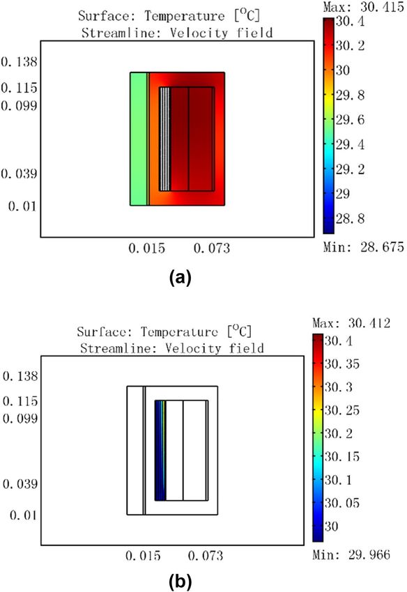
www.nature.com/scientificreports/

                                           Figure 2.  Principle of smart component embedded GMM: (a) embedded GMM smart components (b) zoomed
                                           view of the component corner.

                                            Diameter of       Length of          Diameter of GMM   Length of GMM    Inner diameter of   Outter diameter of
                                            component (mm)    component (mm)     rod (mm)          rod (mm)         driving coil (mm)   driving coil (mm)
                                            30                310                30                60               78                  146

                                           Table 1.  Design parameters of GMM smart component.

                                           Figure 3.  Smart component system.

                                           Model of the GMM smart component
                                           This is a typical fluid model for convective heat transfer. Thus, it is necessary to establish a model involving fluid
                                           coupled heat transfer calculations.

                                           Time‑averaged movement equations of turbulence and convection. It can be assumed that flow-
                                           ing water is in a turbulent state based on the structural parameters of the GMM smart component. Therefore, the
                                           temperature distribution of the GMM smart component is calculated by using the Reynolds-averaged Navier–
                                           Stokes equation (RANS). In the case of turbulent motion, the instantaneous variables of a fixed point (φ ) can be
                                           divided into the average ( φ ) and pulsation (φ ′ ) with φ = φ + φ ′ ; furthermore, the time average of φ ′ is zero. The
                                           average ( φ ) follows these calculation rules 28:

          Scientific Reports |   (2021) 11:251 |                 https://doi.org/10.1038/s41598-020-80460-5                                                      4

Vol:.(1234567890)
www.nature.com/scientificreports/
Figure 4. Smart component testing system.
′
f =f f =0
f +g =f +g f ·g =f ·g
(1)
f ·g = f ·g
f · g = f · g + f ′g ′
∂f ∂f
∂s = ∂s αf = αf
where f and g are two physical quantities, s represents any independent variable, and α is a constant. The time-
averaged movement equations of incompressible turbulence can be obtained from Eq. (1).
Continuity equation. Equation (2) is the continuity equation for incompressible flow.Three variables
below(u, v, w) are the velocity component of the particle in the fluid in the X, Y, and Z directions respectively.
∂u ∂v ∂w
+ + =0 (2)
∂x ∂y ∂z
where u = u + u′ , v = v + v ′ , w = w + w ′ , and Eq. (2) can be substituted by Eq. (3):
∂u ∂v ∂w ∂u′ ∂v ′ ∂w ′
+ + + + + =0 (3)
∂x ∂y ∂z ∂x ∂y ∂z
Using Eq. (1), the time-averaged equation of Eq. (3) can be described as:
∂u ∂v ∂w
+ + =0 (4)
∂x ∂y ∂z
∂u′ ∂v ′ ∂w ′
+ + =0 (5)
∂x ∂y ∂z
Equations (4) and (5) are the continuity equations for incompressible turbulence. We can find the time-
averaged turbulent velocity satisfying the continuity equation.
Movement equation. The average and pulsation are substituted into the Navier–Stokes equation, and then
the time-average is calculated. Thus, the following equation can be obtained:
∂(ρui ) ∂(ρui uj ) ∂p ∂ ∂ui
+ =− + µ − ρui′ uj′ , (i, j = 1, 3) (6)
∂t ∂xj ∂xi ∂xj ∂xj
where ρ is the fluid density. Equation (6) is the time-averaged movement equations of incompressible turbulence.
Energy equation. Omitting the dissipated energy items from the incompressible fluid energy equation and
assuming every physical quantity is represented by the sum of the average and pulsation, we can deduce Eq. (7):
Scientific Reports | (2021) 11:251 | https://doi.org/10.1038/s41598-020-80460-5 5
Vol.:(0123456789)
www.nature.com/scientificreports/
cµ c1 c2 σk σε σT
0.09 1.44 1.92 1.0 1.3 0.9–1.0
Table 2. K − ε model parameters.
∂(T + T ′ ) ∂(T + T ′ ) ∂(T + T ′ )
ρc + ρc(u + u′ ) + ρc(v + v ′ )
∂t ∂x ∂y
(7)
′
′
∂(T + T ) 2
∂ (T + T ) ∂(T + T ′ ) ∂ 2 (T + T ′ )
′
+ ρc(w + w ) = + +
∂z ∂x 2 ∂y 2 ∂z 2
By using Eq. (1), Eq. (7) can be transformed as:
2
∂ 2T ∂ 2T
∂T ∂T ∂T ∂T ∂ T ∂
∂
∂
ρc +pcu +ρcv +ρcw = 2
+ 2
+ 2
− ρcu′ T ′ − ρcv ′ T ′ − ρcw ′ T ′
∂t ∂x ∂y ∂z ∂x ∂y ∂z ∂x ∂y ∂z
(8)
Equation (8) is the energy equation of incompressible turbulence.
K − ε turbulent model. The continuity equation, movement equation, and energy equation are not closed
equations; therefore, we must consider the relationship between additional pulsation and time-average items.
According to the instantaneous Navier–Stokes relationship given by Eq. (9) and Reynolds time-average given by
Eqs. (10, 11) ( K Equation) can be obtained 30.
∂ui ∂ui ∂p ∂ ∂ui ∂uk
ρ + uk =− + µ + (9)
∂t ∂xk ∂xi ∂xk ∂xk ∂xi
∂ui ∂ui ∂p ∂ ∂ui ∂uk
ρ + uk =− + µ + − ρui′ uk′ (10)
∂t ∂xk ∂xi ∂xk ∂xk ∂xi
3
K /2
∂K ∂K ∂ µt ∂K ∂ui ∂ui ∂uj
ρ + ρuj = µ+ + µt + − cD ρ (11)
∂t ∂xj ∂xj σk ∂xj ∂xj ∂xj ∂xi l
where σk is the pulsation momentum’s Prandtl parameter. After using Eq. (11) to determine the fluid viscos-
ity coefficient (µt ), the continuity equation, movement equation, energy equation, and ε Eq. (12) are closed
equations31.
c2 ρε2
∂ε ∂ε ∂ µt ∂ε c1 ε ∂ui ∂ui ∂uk
ρ + ρuj = µ+ + µt + − (12)
∂t ∂xj ∂xj σε ∂xj K ∂xk ∂xk ∂xi K
Using the K − ε model, the fluid viscosity coefficient is shown as Eq. (13) with the parameters listed in Table 2.
1 1
µt = cµ′ ρK 2 l = (cµ′ cD )ρK 2 = cµ ρK 2 /ε (13)
3
cD K /2
Thus, the turbulent convective heat transfer can be calculated by solving the continuity equation, movement
equation, energy equation, K − ε turbulent equations, and Eq. (13).
Results and discussion
Theoretical model simulation. The difference between the GMM and bulk material is ignored; thus, the
thermal structure of the GMM can be considered axially symmetric, as shown in Fig. 5.
In the thermal field analysis of the GMM smart component, the key goal is to conduct an analysis of the
cooling water’s flow-thermal coupling. Through the theoretical analysis discussed in the previous section, Eqs.
(4)–(13) must be solved.
COMSOL Multiphysics software version 5.3 is a professional finite element numerical analysis package. Using
this software, modelling the coupling analysis of physics field combinations can be implemented simultaneously
by selecting different modules. For a temperature field analysis of the GMM smart component, we used one
“ K − ε turbulent model” module and two “General Heat Transfer” modules.
At the inlet, the model is set the velocity component in the z direction, u, to 0.0464 m/s, and that in the r direc-
tion, v, to zero. The model is specified a constant pressure value of 0 at the outlet and logarithmic wall functions
at the solid walls.The model uses two heat transfer application modes: one for the solid and one for the fluid.
These are connected through a heat flux boundary condition, the thermal wall function.
Scientific Reports | (2021) 11:251 | https://doi.org/10.1038/s41598-020-80460-5 6
Vol:.(1234567890)
www.nature.com/scientificreports/

                                 Figure 5.  Thermal analysis model of the GMM smart component.

                                 Figure 6.  For a current of 0.5 A, temperature distribution of GMM smart component under no cooling water.

                                     Based on the flow-thermal coupling finite element models, temperature field simulation analysis was com-
                                 pleted at different inputs under an ambient temperature of 25 °C. The simulation results are shown in Figs. 6,
                                 7, 8, 9.
                                     Figure 6 shows that the coil temperature rose to a maximum of 25.784 °C and the GMM rod temperature rose
                                 to 25.7 °C for a 0.5 A current with no cooling water. When 30 °C cooling water passed through the GMM smart
                                 component, because the water temperature was higher than that of the coil, the coil temperature rose to 30 °C and
                                 the GMM rod temperature rose to 29.5 °C in Fig. 7a. Figure 7b shows that the inlet water temperature was 30 °C,
                                 whereas the temperature at the outlet near the coil was slightly lower at 29.985 °C, which was nevertheless sig-
                                 nificantly higher than 25.784 °C. This indicates that the heat was transferred from 30 °C cooling water to the coil.
                                     Figure 8 shows that the coil temperature rose to a maximum of 53.629 °C and the GMM rod temperature rose
                                 to 50.5 °C for a 3 A current with no cooling water. When 30 °C cooling water passed through the GMM smart
                                 component, the coil maximum temperature was 30 °C, the GMM rod temperature was 29.5 °C, and the container
                                 wall temperature was 30 °C, as shown in Fig. 9a. Figure 9b shows that the inlet water temperature was 30 °C,
                                 whereas the temperature at the outlet near the coil was 30.08 °C. This indicates that heat was transferred from
                                 the coil to the 30 °C cooling water, which ensured that the GMM rod temperature remained constant at 29.5 °C.
                                     From the above analysis, it is clear that the GMM rod temperature stayed at 29.5 °C as long as the cooling
                                 water temperature was 30 °C for an input current of 3 A or less and a flow rate of 0.0464 m/s. This temperature
                                 control can ensure that the GMM remains at a certain temperature, which can eliminate the effects of the drive
                                 coil heating for the precise positioning of the GMM smart component.
                                     For a cooling water temperature of 30 °C, input current of 3 A, and cooling water input flow rates of
                                 0.01 m/s and 0.02 m/s, the temperature distribution of the GMM smart component is shown in Figs. 10 and 11,
                                 respectively.
                                     Figures 9, 10, 11 show that when the input flow rate of the cooling water was 0.0464 m/s, the GMM rod
                                 temperature was 29.5 °C; when the input flow rate of the cooling water was 0.01 m/s, the GMM rod temperature
                                 was 29.6 °C; and when the input flow rate of the cooling water was 0.02 m/s, the GMM rod temperature was

Scientific Reports |   (2021) 11:251 |                https://doi.org/10.1038/s41598-020-80460-5                                                   7

                                                                                                                                              Vol.:(0123456789)
www.nature.com/scientificreports/

                                           Figure 7.  Temperature distribution of GMM smart component for a current of 0.5 A, cooling water
                                           temperature of 30 °C, and flow rate of 0.0464 m/s.

                                           Figure 8.  For a current of 3 A, temperature distribution of GMM smart component with no cooling water.

          Scientific Reports |   (2021) 11:251 |              https://doi.org/10.1038/s41598-020-80460-5                                             8

Vol:.(1234567890)
www.nature.com/scientificreports/

                                 Figure 9.  Temperature distribution of GMM smart component for a current of 3 A, cooling water temperature
                                 of 30 °C, and flow rate of 0.0464 m/s.

                                 29.5 °C. These figures indicate that at a low cooling water flow rate, the heat generated by the driving coil can be
                                 transmitted to the GMM rod. When the cooling water flow rate increases, the heat generated by the driving coil
                                 is removed by the cooling water. The temperature of the GMM rod is completely determined by the temperature
                                 of the cooling water. In this case, if the temperature continues to increase, the water flow rate of the cooling water
                                 flow rate has no effect on the temperature distribution in the GMM rod.

                                 Experimental investigation. The control system of the GMM smart component is designed based on the
                                 simulation results. To reduce the effect of the heat generated by the drive coil and improve the accuracy of radial
                                 displacement required by the GMM smart components, a new forced water cooling control strategy is proposed,
                                 as shown in Fig. 12.
                                     The temperature control system starts heating the water when the temperature is lower than the design
                                 threshold. The water pump starts when the water temperature is at the design threshold. While the GMM smart
                                 component is working, the temperature of the water tank will rise because the cooling water absorbs heat from
                                 the driving coils. When the temperature of the water tank is higher than the design threshold, the temperature
                                 control system will switch on the cooling fan. This control strategy is simple because it ensures a constant cool-
                                 ing water temperature. The temperature control system is not required to change the pump velocity according
                                 to the temperature.
                                     The experimental results of the GMM smart component temperature are shown in Fig. 13. The temperature of
                                 the GMM smart component increased for 450 min and then reached thermal equilibrium with the temperature

Scientific Reports |   (2021) 11:251 |                https://doi.org/10.1038/s41598-020-80460-5                                                     9

                                                                                                                                                Vol.:(0123456789)
www.nature.com/scientificreports/

                                           Figure 10.  GMM smart component temperature distribution for a current of 3 A, cooling water temperature of
                                           30 °C, and flow rate of 0.01 m/s.

                                           remaining constant for a current of 3 A. The temperature of the GMM smart component attained 54.1 °C. The
                                           simulation results shown in Fig. 8 and our experimental results show that the model error is less than 0.9%.
                                               The experimeantal results of the GMM smart components for different input currents and the radial bending
                                           deformation at 25, 30, 40 and 50 °C cooling water are shown in Fig. 14.When the cooling water temperature rises
                                           from 25 to 30 °C, the radial bending deformation of GMM smart components with current decreases, but the
                                           decrease amount is very small, and the two are basically the same. When the temperature rises from 30 to 40 °C,
                                           the radial bending deformation of the GMM smart component increases. when the temperature rises from 40
                                           to 50 °C, the radial bending deformation of the GMM smart component decrease.The maximum radial bending
                                           deformation of the component occures at 40 °C cooling water and is 441 μm.
                                               Table 3 shows a comparison of the simulation and experimental results for an ambient temperature of 25 °C
                                           and input currents of 0.5, 2, and 3 A using 30 °C cooling water to cool the GMM smart component. The cooling
                                           water flow rate was 0.0464 m/s. After 10 min of cooling, the temperature of the GMM smart component was
                                           measured.
                                               Table 3 shows that the difference between the simulation result and measured value does not exceed 0.3 °C,
                                           and the maximum error is 1%.
                                               Furthermore, Table 4 shows a comparison of the simulation and experimental results for an ambient tem-
                                           perature of 25 °C and cooling water flow rates of 0.01, 0.02, and 0.0464 m/s using 30 °C cooling water to cool
                                           the GMM smart component. The input current was 3 A. After 10 min of cooling, the temperature of the GMM
                                           smart component was measured.
                                               Table 4 shows that the difference between the simulation result and the measured value does not exceed 0.4 °C,
                                           and the maximum error is 1.33%. A comparison of the simulation results and experimental results illustrates that

          Scientific Reports |   (2021) 11:251 |                https://doi.org/10.1038/s41598-020-80460-5                                                10

Vol:.(1234567890)
www.nature.com/scientificreports/
Figure 11. GMM smart component temperature distribution for a current of 3 A, cooling water temperature of
30 °C, and flow rate of 0.02 m/s.
Figure 12. Schematic diagram of new control system for GMM smart component.
the flow-thermal coupling model of the GMM smart component is correct, but it also shows that the selected
temperature control is effective.
Conclusions
Focusing on the impact of the thermal effect on the performance of GMM smart components, a new simplified
control strategy is proposed to ensure a constant GMM temperature. Our study can be summarized as follows:
Scientific Reports | (2021) 11:251 | https://doi.org/10.1038/s41598-020-80460-5 11
Vol.:(0123456789)www.nature.com/scientificreports/
Figure 13. For current 3 A, temperature of GMM smart component rised with time is observed under no
cooling water.
Figure 14. The radial bending deformation of GMM smart component vared with currents under various
temperature cooling water.
Input current (A) Simulation result (°C) Measurement result (°C)
0.5 30 30.1
2 30 30.3
3 30 30.2
Table 3. Comparison of simulation results and experimental results at different input currents.
Cooling water flow rate (m/s) Simulation results (°C) Measurement results (°C)
0.01 30 30.4
0.002 30 30.2
0.0464 30 30.1
Table 4. Comparison of simulation results and experimental results at different cooling water flow rates.
Scientific Reports | (2021) 11:251 | https://doi.org/10.1038/s41598-020-80460-5 12
Vol:.(1234567890)www.nature.com/scientificreports/
1. Our strategy involves establishing and implementing a turbulent flow-thermal coupling finite element model
for the GMM smart component by applying flow-thermal coupling theory.
2. Our strategy only involves maintaining the cooling water at a certain temperature and does not control the
flow rate to eliminate the effects of the drive coil heating elements for precise positioning of the GMM smart
component.
3. The control system of the GMM smart component is developed and implemented. When the input current
is 3 A, the GMM smart component temperature attains 54.1 °C, while the simulation result is 53.629 °C. The
error is within 0.9%. Thus, the experimental results indicate that the flow-thermal coupling model for the
GMM smart component is appropriate.
4. When the input current of the GMM smart component is 0.5, 2, or 3 A, the cooling water flow rate is
0.0464 m/s. The cooling water is used to cool the component. The difference between the simulation result
and actual measurement does not exceed 0.3 °C; thus, the maximum error is 1%. When the input current
is 3 A, the cooling water flow rates are 0.01, 0.02, and 0.0464 m/s, with 30 °C cooling water used to cool the
GMM smart component. The difference between the simulation result and the measured value does not
exceed 0.4 °C; thus, the maximum error is 1.33%. This indicates that the selected temperature control is
effective.
However, the entire temperature-rise control system has a large volume structure, which is not suitable for
the application of GMM devices in a narrow space. Therefore, it is necessary to further explore the temperature
rise control method using simple structures with a small volume, which would ensure that the GMM device
could be more widely used.
Received: 3 October 2020; Accepted: 18 December 2020
References
1. Gao, X., Liu, Y., Guo, H. & Yang, X. Structural design of giant magnetostrictive actuator. AIP Adv. 8, 065211–065219. https://doi.
org/10.1063/1.5030753 (2018).
2. Zheng, X. & Sun, L. A one-dimension coupled hysteresis model for giant magnetostrictive materials. J. Magn. Magn. Mater. 309,
263–271. https://doi.org/10.1016/j.jmmm.2006.07.009 (2007).
3. Zhu, Y. & Ji, L. Theoretical and experimental investigations of the temperature and thermal deformation of a giant magnetostrictive
actuator. Sens. Actuators A 218, 167–178. https://doi.org/10.1016/j.sna.2014.07.017 (2014).
4. Yang, Z. et al. Direct drive servo valve based on magnetostrictive actuator: Multi-coupled modeling and its compound control
strategy. Sens. Actuators A 235, 119–130. https://doi.org/10.1016/j.sna.2015.09.032 (2015).
5. Yu, C., Wang, C., Deng, H., He, T. & Mao, P. Hysteresis nonlinearity modeling and position control for a precision positioning
stage based on a giant magnetostrictive actuator. RSC Adv. 6, 59468–59476. https://doi.org/10.1039/c6ra05195b (2016).
6. Witthauer, A., Kim, G. Y., Faidley, L., Zou, Q. & Wang, Z. Design and characterization of a flextensional stage based on terfenol-D
actuator. Int. J. Precis. Eng. Manuf. 15, 135–141 (2014).
7. Zhang, K. et al. Magnetostrictive resonators as sensors and actuators. Sens. Actuators A 200, 2–10. https://doi.org/10.1016/j.
sna.2012.12.013 (2013).
8. Liu, H., Ma, K., Liang, Q., Gu, Y. & Wang, H. Temperature characteristics of GMA and passive compensation method for its thermal
deformation GMA. Zhendong yu Chongji/J. Vib. Shock 38, 149–156. https://doi.org/10.13465/j.cnki.jvs.2019.15.021 (2019).
9. Xia, C. L., Ding, F. & Tao, G. Experimental study on thermal deformation compensation of giant magnetostrictive electro-mechan-
ical converter. China Mech. Eng. 10, 563–565 (1999).
10. Yu, Z. Study on thermal deformation compensation based on giant magnetostrictive material actuator for servo valve. J. China
Coal Soc. 31, 396–400. https://doi.org/10.1007/s11434-006-2076-2 (2006).
11. Yamamoto, Y., Eda, H. & Shimizu, J. in 1999 IEEE/ASME. International Conference on Advanced Intelligent Mechatronics. 215–220
(IEEE).
12. Wang, H. Study on Thermal Characteristics and Thermal Deformation Compensation of Giant Magnetostrictive Actuator(Master
thesis) Master thesis thesis, Shenyang University of Technology, (2017, pp. 37–45).
13. Yan, R. G., Zhu, L. H. & Dong, X. X. Design of a giant magnetostrictive actuator and research on the effect of water cooling system.
Adv. Mater. Res. 889–890, 893–896. https://doi.org/10.4028/www.scientific.net/AMR.889-890.893 (2014).
14. Jia, Y. & Tan, J. Study on micro-position actuator system of giant magnetostrction materials. Chin. J. Sci. Instrum. 021, 38–41
(2001).
15. Lu, Q., Jing, C., Min, Z., Chen, D. & Cao, Q. in International Conference on Mechanic Automation and Control Engineering (MACE).
3562–3565.
16. Lu, Q., Chen, D., Zhong, Y. & Chen, M. Research on thermal deformation and temperature control of giant magnetostrictive
actuator. China Mech. Eng. 18, 16–19 (2007).
17. Simons, R. E. & Chu, R. C. in Semiconductor Thermal Measurement and Management Symposium. 1–9 (IEEE).
18. Xu, J., Wu, Y., Zhao, Z. R. & Ge, R. J. The design of temperature control system in giant magnetostrictive actuator. Mod. Mach. Tool
Autom. Manuf. Techn. 10, 47–49 (2007).
19. Fan, Z., Lou, J. & Zhu, S. in 3rd international Conference on Manufacturing Science and Engineering. 2600–2604 (Trans Tech
Publications).
20. Liu, C. Application of phase change temperature control to GMA. Mod. Mach. Tool Autom. Manuf. Tech. 10, 50–52 (2006).
21. Wu, Y. & Xu, J. Research on methods of thermal error compensating and restraining in giant magnetostrictive actuator. J. Eng.
Des. 12, 213–218 (2005).
22. Ahanpanjeh, M., Ghodsi, M. & Hojjat, Y. Precise positioning of terfenol-D actuator by eliminating the heat generated by coil. Mod.
Appl. Sci. 10, 232–244. https://doi.org/10.5539/mas.v10n9p232 (2016).
23. Goulbourne, N. C. et al. in SPIE Smart Structures and Materials + Nondestructive Evaluation and Health Vol. 9800 980008 (2016).
24. Zhang, C. & Zhang, H. Modling and comepensation of thermal characteristics of giant magnetosrictive material. J. Qufu Norm.
Univ. 46, 99–102 (2020).
25. Ji, L., Zhu, Y., Yang, X., Fei, S. & Guo, Y. Theoretical analysis and experiment of power loss in giant magnetostrictive actuator. J.
Aerosp. Power 32, 1066–1073. https://doi.org/10.13224/j.cnki.jasp.2017.05.006 (2017).
26. Kwak, Y. K., Kim, S. H. & Ahn, J. H. Improvement of positioning accuracy of magnetostrictive actuator by means of built-in air
cooling and temperature control. Int. J. Precis. Eng. Manuf. 12, 829–834. https://doi.org/10.1007/s12541-011-0110-z (2011).
Scientific Reports | (2021) 11:251 | https://doi.org/10.1038/s41598-020-80460-5 13
Vol.:(0123456789)www.nature.com/scientificreports/
27. Zhao, T., Yuan, H., Pan, H. & Li, B. Study on the rare-earth giant magnetostrictive actuator based on experimental and theoretical
analysis. J. Magn. Magn. Mater. 460, 509–524 (2018).
28. Bo, S., Zhang, Z. & Yan, H. Water immersion cooling technology of rare earth giant magnetostrictive actuator. J. Mech. Electr. Eng.
36, 842–845 (2019).
29. Wu, Y. & Xiang, Z. Machining principle for non-cylinder pin hole of piston based on giant magnetostrictive material. J. Zhejiang
Univ. Sci. A Sci. Eng. 38, 213–218. https://doi.org/10.1007/s11766-004-0013-1 (2004).
30. Tao, W. Numerical heat transfer. Vol. 10 347–353 (Xi’an Jiaotong University Press, 2001, pp. 347–353).
31. Hou, H., Wei, Q. & Zhang, Z. Numerical simulation on the turbulent flow and heat transfer characteristics of offset-strip-fin
compact heat exchanger. Energy Eng. 6, 6–10 (2002).
Acknowledgements
This research was partially funded by the Beijing Key Laboratory of Logistics Systems.
Author contributions
Zhao Z.R. wrote the main manuscript text and Sui X.M. reviewed the manuscript.
Funding
This work was supported by the Scientific Research Plan of Beijing Education Commission (KM202010037001),
the National Natural Science Foundation of China (Grant Number 31470588), and the Research Topics of China
Logistics Association and China Federation of Logistics and Purchasing (2019CSLKT3-119).
Competing interests
The authors declare no competing interests.
Additional information
Correspondence and requests for materials should be addressed to X.S.
Reprints and permissions information is available at www.nature.com/reprints.
Publisher’s note Springer Nature remains neutral with regard to jurisdictional claims in published maps and
institutional affiliations.
Open Access This article is licensed under a Creative Commons Attribution 4.0 International
License, which permits use, sharing, adaptation, distribution and reproduction in any medium or
format, as long as you give appropriate credit to the original author(s) and the source, provide a link to the
Creative Commons licence, and indicate if changes were made. The images or other third party material in this
article are included in the article’s Creative Commons licence, unless indicated otherwise in a credit line to the
material. If material is not included in the article’s Creative Commons licence and your intended use is not
permitted by statutory regulation or exceeds the permitted use, you will need to obtain permission directly from
the copyright holder. To view a copy of this licence, visit http://creativecommons.org/licenses/by/4.0/.
© The Author(s) 2021
Scientific Reports | (2021) 11:251 | https://doi.org/10.1038/s41598-020-80460-5 14
Vol:.(1234567890)You can also read