TASM: A Tile-Based Storage Manager for Video Analytics
←
→
Page content transcription
If your browser does not render page correctly, please read the page content below
TASM: A Tile-Based Storage Manager for Video
Analytics
Maureen Daum∗ , Brandon Haynes† , Dong He∗ , Amrita Mazumdar∗ , Magdalena Balazinska∗
∗ Paul G. Allen School of Computer Science & Engineering, University of Washington
{mdaum, donghe, amrita, magda}@cs.washington.edu
† Gray Systems Lab, Microsoft
Brandon.Haynes@microsoft.com
Abstract—Modern video data management systems store
videos as a single encoded file, which significantly limits possible
storage level optimizations. We design, implement, and evaluate
TASM, a new tile-based storage manager for video data. TASM
uses a feature in modern video codecs called “tiles” that enables
spatial random access into encoded videos. TASM physically
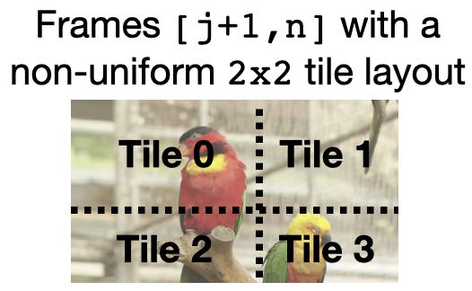
tunes stored videos by optimizing their tile layouts given the video (a) (b) (c)
content and a query workload. Additionally, TASM dynamically Fig. 1. Video partitioned into tiles. (a) shows the first j frames partitioned
tunes that layout in response to changes in the query workload with a uniform 1×2 layout. (b) shows frames partitioned with a non-
or if the query workload and video contents are incrementally uniform 2×2 layout. (c) shows a directory hierarchy. Video stored at
discovered. Finally, TASM also produces efficient initial tile video/frames_1-j/tile0.mp4 contains the left half of frames [1, j].
layouts for newly ingested videos. We demonstrate that TASM
can speed up subframe selection queries by an average of over of reading and decoding the video file is known to significantly
50% and up to 94%. TASM can also improve the throughput of hurt the performance of this phase [13].
the full scan phase of object detection queries by up to 2×. In this paper, we introduce TASM, a storage manager that
greatly improves the performance of subframe selection queries
I. I NTRODUCTION
and the full scan phase of object detection queries by providing
The proliferation of inexpensive high-quality cameras spatial random access within videos. TASM exploits the
coupled with recent advances in machine learning and computer observation that objects in videos frequently lie in subregions
vision have enabled new applications on video data such as of video frames. For example, a traffic camera may be oriented
automatic traffic analysis [1], [2], retail store planning [3], and such that it partially captures the sky, so vehicles only appear
drone analytics [4], [5]. This has led to a class of database in the lower portion of a frame. Analysis applications such
systems specializing in video data management that facilitate as running license plate recognition [1] or extracting image
query processing over videos [3], [6]–[10]. patches for vehicle type recognition [1] only need to operate on
A query over a video comprises two steps. First, read the parts of the frame containing vehicles. Privacy applications
the video file from disk and decode it. Second, process such as blurring license plates and faces [14] or performing
frames to identify and return pixels of interest or compute an region of interest-based encryption [15] similarly only need to
aggregate. Most systems, so far, have focused on accelerating modify the parts of the frame that contain sensitive objects.
and optimizing the second step [3], [9]–[11], often assuming Using its spatial random access capability, TASM enables
that the video is already decoded and stored in memory [3], reading from disk and decoding only the parts of the frame
[7], [12], which is not feasible in practice. that are interesting to queries. Providing such a capability is
The lack of efficient storage managers in existing video difficult because the video encoding process introduces spatial
data management systems significantly impacts queries. First, and temporal dependencies within and between frames. To
subframe selection queries (e.g., “Show me video snippets address this problem, TASM subdivides video frames into
cropped to show previously identified hummingbirds feeding on smaller pieces called tiles that can be processed independently.
honeysuckles” ) are common and their execution bottleneck is at As shown in Fig. 1, each tile contains a rectangular subregion
the storage layer since these queries are selections, reading and of the frame that can be decoded independently because there
returning pixels without additional operations. Second, object are no spatial dependencies between tiles. In contrast, current
detection queries, which extract new semantic information state of the art incurs the cost of decoding entire frames. TASM
from a video (e.g., “Find all sightings of hummingbirds in this optimizes how a video is divided into tiles and stored on disk to
new video”) require the execution of expensive deep learning reduce the amount of work spent decoding and preprocessing
models. To avoid applying such models to as many frames as parts of the video not involved in a query. Through its use of
possible, query plans typically include an initial full scan phase tiles, TASM implements a new type of optimization that we
that applies a cheap predicate [12] or a specialized model [7] call semantic predicate pushdown where predicates are pushed
to the entire video to filter uninteresting frames. The overhead below the decoding step and only tiles of interest are read from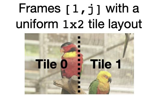
disk, decoded, and processed.                                       object detection query is executed, TASM only decodes the
   Building TASM raises three challenges. The first challenge       tiles that contain ROIs, hence filtering regions of the frame
is fundamental, but important: Given a video file with known        before the decode step. TASM thus alleviates the bottleneck
semantic content (i.e., known object locations within video         for the full scan phase of object detection queries by reducing
frames) and a known query workload, TASM must decide on             the amount of data that must be decoded and preprocessed.
the optimal tile layout, choosing from among layouts with           TASM can be directly incorporated into existing techniques and
uniform or non-uniform tiles and either fine-grained or coarse-     systems that accelerate the extraction of semantic information
grained tiles. TASM must also decide whether different tile         from videos (e.g., [3], [11]).
layouts should be used in different parts of a video. To do            In summary, the contributions of this paper are as follows:
this effectively, TASM must accurately estimate the cost of                                    1
                                                                       • We develop TASM , a new type of storage manager for
executing a query with a given tile layout. TASM therefore                video data that splits video frames into independently
drives its selection using a cost function that balances the              queryable tiles. TASM optimizes the tile layout of a
benefits of processing fewer pixels against the overhead of               video file based on its contents and the query workload.
processing more tiles for a given tile layout, video content, and         By doing so, TASM accelerates queries that retrieve
query workload. In this paper, we experimentally demonstrate              objects in videos while keeping storage overheads low
that non-uniform, fine-grained tiles outperform the other                 and maintaining good video quality.
options. Additionally, we find that optimizing the layout for          • We develop new algorithms for TASM to dynamically
short sections of the video (i.e., every 1 second) maximizes              evolve the video layout as information about the video
query performance with no storage overhead. Given a video                 content and query workload becomes available over time.
file, TASM thus splits it into 1 second fragments and selects
                                                                       • We extend TASM to cheaply profile videos and design
the optimal fine-grained tile layout for each fragment.
                                                                          an initial layout around ROIs when a video is initially
   The second challenge is that the semantic content and the
                                                                          ingested. This initial tiling reduces the preprocessing work
query workload for a video are typically discovered over time
                                                                          required for object detection queries.
as users execute object detection and subframe selection queries.
TASM therefore lacks the information it needs to design optimal        We evaluate TASM on a variety of videos and workloads
tile layouts. To address this challenge, TASM incrementally         and find that the layouts picked by TASM speed up subframe
updates a video’s tile layout as queries to detect and retrieve     selection queries by an average of 51% and up to 94%
objects are executed. TASM uses different tile layouts in           while maintaining good quality, and that TASM automatically
different parts of the video, and independently evolves the tile    tunes layouts after just a small number of queries to improve
layout in each section. To do this, TASM builds on techniques       performance even when the workload is unknown. We also find
from database cracking [16], [17] and online indexing [18].         that TASM improves the throughput of the full scan phase of
To decide when to re-tile portions of the video and which           object detection by up to 2× while maintaining high accuracy.
layout to use, TASM maintains a limited set of alternative
layouts based on past queries. It then uses its cost function to                               II. BACKGROUND
accumulate estimated performance improvements offered by               Videos are stored as encoded files due to their large size.
these tile layouts as it observes queries. Once the estimated       Video codecs such as H264 [20], HEVC [21], and AV1 [22]
improvement, also called regret [19], of a new layout offsets       specify algorithms used to (de)compress videos. While the
the cost of reorganization, TASM re-tiles that portion of the       specific algorithms used by various codecs differ, the high-
video. By observing multiple queries before making tiling           level approach is the same as we describe in this section.
decisions, TASM designs layouts optimized for multiple query           Groups of pictures: A video consists of a sequence of
types. For the ornithology example, TASM could tile around          frames, where each frame is a 2D array of pixels. Frames in
hummingbirds and flowers that are likely to attract them.           the sequence are partitioned into groups of pictures (GOPs).
   The third challenge lies in the initial phase that identifies    Each GOP is encoded independently from the other GOPs
objects of interest in a new video. This phase is both expensive    and is typically one second in duration. The first frame in a
and requires at least one full scan over the video, generally       GOP is called a keyframe. Keyframes allow GOPs to act as
using a cheap model to filter frames or compute statistics.         temporal random access points into the video because it is
The models used in the full scan phase are limited by video         possible to start decoding a video at any keyframe. To retrieve
decoding and preprocessing throughput [13]. To address this         a specific frame, the decoder begins decoding at the closest
final challenge, TASM uses semantic predicate pushdown where        keyframe preceding the frame being retrieved. Keyframes have
the semantic predicate is not a specific object type, but rather    large storage sizes because they use a less efficient form of
a general region of interest (ROI). TASM bootstraps an initial      compression than other types of frames, so the number of
tile layout using an inexpensive predicate that identifies ROIs     keyframes impacts a video’s overall storage size. Videos stored
within frames. This predicate can use background segmentation       with long GOPs are smaller in size than videos stored with short
to find foreground objects, motion vectors to identify areas        GOPs, but they also have fewer random access opportunities.
with large amounts of motion, or even a specialized neural
network designed to identify specific object types. When an           1 Code   is available at https://github.com/uwdb/TASM.
Tiles: Compressed videos do not generally support decoding
spatial regions of a frame. The encoding process creates spatial
dependencies within a frame, and decoders must resolve these
dependencies by decoding the entire frame, even if just a small
region is requested. Modern codecs, however, provide a feature
called tiles that enables splitting frames into independently-
decodable regions. Fig. 1 illustrates this concept. Like frames,
tiles are also 2D arrays of pixels. However, a tile only contains Fig. 2. Overview of how TASM integrates with a VDBMS.
the pixels for a rectangular portion of the frame. The full frame
is recovered by combining the tiles. Tiles introduce spatial index to store the bounding boxes associated with object
random access points for decoding. To decode a region within detections. While queries for statistics about the semantic
a frame, only the tiles that contain the requested region are content can use the semantic index to avoid re-running
processed. This flexibility to decode spatial subsets of frames expensive analysis over the frame contents, TASM uses this
comes with tradeoffs in quality; tiling can lead to artifacts index to generate tile layouts, split videos into tiles, store such
appearing at the tile boundaries [23], which reduces the visual physically tuned videos as files, and answer content-based queries
quality of videos. As such, carefully selecting tile layouts is more efficiently by retrieving only relevant tiles from disk.
important for high-quality query results. While tiles act as spatial
random access points, temporal random access is still provided A. TASM API
by keyframes. Tiles are applied to all frames within a GOP, so TASM exposes the following access method API:
decoding a tile in a non-keyframe requires decoding that tile in
Method Parameters Result
all frames starting from the preceding keyframe.
A tile layout defines how a sequence of frames is divided S CAN video, L : labels, T : times Pixel[]
into tiles. A layout L= (nr , nc , {h1 , . . . , hnr }, {w1 , . . . , wnc }) A DD M ETADATA video, f rame, label, —
is defined by the number of rows and columns, nr and nc , x1 , y 1 , x 2 , y 2
the height of each row, and the width of each column. These
The core method S CAN (video, L, T ) performs subframe
parameters define the (x, y) offset, width, and height of the
selection by retrieving the pixels that satisfy a CNF predicate on
nr ·nc tiles. An untiled video is a special case of a tile layout
the labels, L, and an optional predicate on the time dimension,
consisting of a single tile that encompasses the entire frame:
T . For example, L=(label=‘car’)∨(label=‘bicycle’) retrieves
ω = (1, 1, {f rame height}, {f rame width}). Valid layouts
pixels for both cars and bicycles.
require tiles to be partitioned along a regular grid, meaning
TASM also exposes an API to incorporate metadata
rows and columns extend through the entire frame. We do
generated during query processing into the semantic
not consider irregular layouts, which are not supported by the
index (discussed in the following section). The method
HEVC specification [21]. Different tile layouts can be used
A DD M ETADATA (video, f rame, label, x1 , y1 , x2 , y2 ) adds the
throughout the video; a sequence of tiles (SOT) refers to a
bounding box (x1 , y1 , x2 , y2 ) on f rame to the semantic index
sequence of frames with the same tile layout. Changes in the
and associates it with the specified label.
tile layout must happen at GOP boundaries, so every new layout
must start at a keyframe. Therefore, changing the tile layout
B. Semantic index
has a high storage overhead for the same reason that starting a
new GOP has a high storage overhead. The cost of executing TASM maintains metadata about the contents of videos in
a query over a video encoded with tiles is proportional to the a semantic index. The semantic information consists of labels
number of pixels and tiles that are decoded. associated with bounding boxes. Labels denote object types
Stitching: Tiles can be stored separately, but they must be and properties such as color. Bounding boxes locate an object
combined to recover the original video. Tiles can be combined within a frame. When the query processor invokes TASM’s
without an intermediate decode step using a process called S CAN method, TASM must efficiently retrieve bounding box
homomorphic stitching [24]. Homomorphic stitching interleaves information associated with the specified parameters. The
the encoded data from each tile and adds header information semantic index is therefore implemented as a B-tree clustered
so the decoder knows how the tiles are arranged. on (video, label, time). The leaves contain information about
the bounding boxes and pointers to the encoded video tile(s)
III. T ILE - BASED STORAGE MANAGER DESIGN each box intersects based on the associated tile layout.
In this section, we present the design of TASM, our tile- The semantic index is populated through the A DD M ETADATA
based storage manager. TASM is designed to be the lowest method as object detection queries execute. As we discuss in
layer in a VDBMS. Unlike existing storage managers that serve Section IV, TASM creates an initial layout around high-level
requests for sequences of frames, TASM efficiently retrieves regions of interest within frames to speed up object detection
regions within frames to answer queries for specific objects. queries. As those queries execute and add more objects to the
Fig. 2 shows an overview of how TASM integrates with the semantic index, TASM incrementally updates the tile layout
rest of a VDBMS. TASM incrementally populates a semantic to maximize the performance of the observed query workload.(a) Uniform 2x4 layout (b) Layout around cars & people
(c) Tile layout around cars (d) Tile layout around people (a) Long layout duration (b) Short layout duration
Fig. 3. Various ways to tile a frame. (a) is a uniform layout, while (b)-(d) Fig. 5. (a) shows how more pixels must be decoded on each individual frame
are non-uniform layouts. Depending on which objects are targeted, different when a tile layout extends for many frames compared to (b) where fewer
layouts will be more efficient. frames have the same layout. The boxes show the location of the car on later
frames, and the dashed lines show the tile boundaries. The striped region
indicates the tile that would be decoded for a query targeting cars.
specified by the codec and ensuring that no tile boundary
intersects any b ∈ B. TASM does not limit the number of tiles
(a) Fine-grained tiles (b) Coarse-grained tiles
in a layout. To modulate quality, this could be made a user-
Fig. 4. Non-uniform tile layout around cars using (a) fine-grained tiles, or (b) specified setting; we leave this as future work. TASM processes
coarse-grained tiles.
fewer pixels from a video stored with fine-grained tiles because
C. Tile-based data storage the tiles do not contain the parts of the frame between objects,
Having captured the metadata about objects and other but it processes more individual tiles because multiple tiles in
interesting areas in a video using the semantic index, the next each frame may contain objects. TASM estimates the overall
step is to leverage it to guide how the video data is encoded effectiveness of a layout using a cost function that combines
with tiles. Two tiling approaches are possible: uniform-sized these two metrics, as described in Section IV-A.
tiles, or non-uniform tiles whose dimensions are set based In addition to deciding the tile granularity, TASM also
on the locations of objects in the video. Both techniques can chooses which objects to design the tile layout around, and
improve query performance, but tile layouts that are designed therefore which bounding boxes to include in B. The best
around the objects in frames can reduce the number of non- choice depends on the queries. For example, if queries target
object pixels that have to be decoded. Fig. 3 shows these people, a layout around just people, as in Fig. 3d, is more
different tiling strategies on an example frame. efficient than a layout around both cars and people (Fig. 3b).
1) Uniform layouts: The uniform layout approach divides We explain how TASM makes this choice in Section IV.
frames into tiles with equal dimensions. This approach does 3) Temporally-changing layouts: Different tile layouts,
not leverage the semantic index, but if objects in the video are uniform and non-uniform, can be used throughout a video; the
small relative to the total frame size, they will likely lie in a layout can change as often as every GOP. TASM uses different
subset of the tiles. However, an object can intersect multiple layouts throughout a video to adapt to objects as they move.
tiles, as shown in Fig. 3a where part of the person lies in two The size of these temporal sections is determined by the
tiles. While TASM decodes fewer pixels than the entire frame, layout duration, which refers to the number of frames within a
it still must process many pixels that are not requested by sequence of tiles (SOT). Layout duration is separate from GOP
the query. Further, the visual quality of the video is reduced length; while layout duration cannot be shorter than a GOP, it
because in general a large number of uniform tiles are required can extend over multiple GOPs. The layout duration affects
to improve query performance, as shown in Fig. 7b. the sizes of tiles in non-uniform layouts, as shown in Fig. 5. In
2) Non-uniform layouts: TASM creates non-uniform layouts general, longer tile layout durations have lower storage costs
with tile dimensions such that objects targeted by queries lie but lead to larger tiles because TASM must consider more
within a single tile. There are a number of ways a given tile object bounding boxes as objects move and new objects appear.
layout can benefit multiple types of queries. If a large portion Therefore, TASM must decode more data on each frame. We
of the frame does not contain objects of interest, the layout can evaluate this tradeoff in Fig. 10.
be designed such that this region does not have to be processed. 4) Not tiling: Layouts that require TASM to decode a similar
If objects of interest appear near each other, a single tile around number of pixels as when the video is not tiled can actually
this region benefits queries for any of these objects. If objects slow queries down due to the implementation complexities that
are not nearby but do appear in clusters, creating a tile around arise from working with multiple tiles. Therefore, TASM may
each cluster can also accelerate queries for these objects. opt to not tile GOPs when the gain in performance does not
Fig. 4 shows examples of non-uniform layouts around cars. exceed a threshold value.
For a set of bounding boxes B, TASM picks tile boundaries 5) Data storage and retrieval: TASM stores each tile as a
guided by a desired tile granularity. For coarse-grained tiles separate video file, as shown in Fig. 1. If different layouts are
(Fig. 4b), it places all B within a single, large tile. For fine- used throughout the video, each tile video contains only the
grained tiles (Fig. 4a), it attempts to isolate non-intersecting b ∈ frames with that layout. If only a segment of a video is ever
B into smaller tiles while respecting minimum tile dimensions queried, TASM reads and tiles just the frames in that segment.This storage structure facilitates the ingestion of new videos Finally, the cost of executing q over video v encoded
because each video’s data is stored separately. Additionally, with layout specification L is the sum of its SOT costs (i.e.,
because each GOP is also stored separately, to modify an C(v, q, L )= si ∈v C(si , q, L (si ))) and the cost of executing
P
existing video, updated GOPs can replace original ones, or an entire queryP workload is the sum over all individual queries,
new GOPs can be appended. C(v, Q, L )= qi ∈Q C(v, qi , L ). The difference in estimated
TASM retrieves just the tiles containing the objects targeted query time for query q over SOT s between layouts L and L0 is
by queries. When complete frames are requested, TASM applies ∆(q, L, L0 , s)=C(s, q, L)−C(s, q, L0 ), or simply ∆(q, L, L0 )
homomorphic stitching (see Section II). This stitching process when s is obvious from the context. The cost of (re-)encoding
can also be used to efficiently convert the tiles into a codec- SOT s with layout L is R(s, L).
compliant video that other applications can interact with. Using this cost function, the maximum expected
improvement for an individual query is inversely proportional to
IV. T ILING STRATEGIES
the object density, which determines the number of pixels (P )
TASM automatically tunes the tile layout of a video to improve and tiles (T ). Tiling therefore leads to negligible improvement—
query performance. The objects in a video and workloads, or the or even regressions—when objects are dense and occupy a large
set of queries presented to a VDBMS, may be known or unknown. fraction of a frame. In those cases, TASM does not tile a video
When TASM has full knowledge of both the objects targeted by at all as we discuss in Section IV-B. In contrast, tiling yields
queries and the locations of these objects in video frames, TASM large improvements when objects are sparse. Fig. 11 shows the
designs tile layouts before queries are processed, as described in linear relationship. It shows how, for a given video and query,
Section IV-B. In practice, the objects targeted by queries and non-uniform tiling reduces the number of pixels that must
their locations are initially unknown. TASM uses techniques be decoded, which directly increases performance. TASM’s
from online indexing to incrementally design layouts based on regret-based approach described in Section IV-C converges to
prior queries and the objects detected so far, as described in such good layouts over time as queries are executed. Fig. 9
Section IV-C. Finally, TASM also creates an efficient, initial tiling also shows how object densities affect performance.
before any queries are executed as we present in Section IV-D.
A. Notation and cost function B. Known queries and known objects
We first introduce notation that will be used throughout We first present TASM’s fundamental video layout
this section. A query workload Q = (q1 , ..., qn ) is a list of optimization assuming a known workload, meaning that TASM
queries, where each query requests pixels belonging to specified knows which objects will be queried, and the semantic index
object classes, possibly with temporal constraints. The set Oqi contains their locations. These assumptions are unlikely to hold
represents the objects requested by an individual query qi , in practice, and we relax them in the next section.
while OQ = ∪qi ∈Q Oqi is the set of all objects targeted by Q. Given a workload and a complete semantic index, TASM
A video v = s0 ⊕ · · · ⊕ sn is a series of concatenated, decides on SOT boundaries then picks a tile layout for each
non-overlapping, non-empty sequence of tiles (SOTs; see SOT to minimize execution costs over the entire workload.
Section II), si . A video layout specification L =si 7→ L More formally, the goal is to partition a video into SOTs,
maps each SOT to a tile layout, L, which specifies how v = s0 ⊕ · · · ⊕ sn and find L ∗ = arg minL C(v, Q, L ).
frames are partitioned into tiles, as described in Section II. The experiment in Fig. 10 motivates us to create small SOTs
If a SOT is not tiled, then si 7→ω, where ω refers to a 1×1 because they perform best. We therefore partition the video
tile layout. PARTITION(s, O) refers to tiling the SOT using a such that each GOP corresponds to a SOT in the tiled video.
non-uniform layout around the bounding boxes associated with This produces a tiled video with a similar storage cost as the
objects in the set O using the techniques from Section III-C2. untiled video because it has the same number of keyframes.
For example, PARTITION(s, {car, person}) refers to creating It would be too expensive for TASM to consider every
a layout around cars and people, as in Fig. 3b. possible layout, uniform and non-uniform, for a given SOT.
TASM implements a “what-if” interface [25] to estimate However, tile layouts that isolate the queried objects should
the cost of executing queries with alternative layouts using a improve performance the most. Additionally, we empirically
cost function. The estimated cost of executing query q over demonstrate that non-uniform layouts outperform uniform
SOT s encoded with layout L is C(s, q, L)=β · P (s, q, L) + γ · layouts (see Fig. 7a), and that fine-grained layouts outperform
T (s, q, L). The cost C is proportional to the number of pixels coarse-grained layouts (see Fig. 9). Therefore, for each si ,
P , and the number of tiles T that are decoded, both of which TASM only considers a fine-grained, non-uniform layout around
depend on the query and layout. To validate this cost function the objects targeted by queries in that SOT, Osi ⊆ OQ .
and estimate β and γ to use in experiments, we fit a linear TASM’s optimization process proceeds in two steps. First, for
model to the decode times for over 1,400 video, query, and each si and associated layout, L=PARTITION(si , Osi ), TASM
non-uniform layout combinations used in the microbenchmarks estimates if re-tiling the SOT with L will improve query
in Section V-B. The resulting model achieves R2 =0.996. The performance at all. As described in Section III-C4, TASM
exact values of β and γ will depend on the system; TASM can does not tile si when P (si , Q, L)>α·P (si , Q, ω), where α
re-estimate them by generating a number of layouts from a small specifies how much a tile layout must reduce the amount of
sample of videos and measuring execution time. decoding work compared to an untiled video (i.e., L=ω). In ourj
1: OQ0 ← ∅, Lalt ← ∅, ∀sj ∈ v : δ j ← 0, L0 ← ω observation that many applications query for similar objects
2: for all qi ∈ Q do
3: OQ0 ← OQ0 ∪ Oqi over time. TASM therefore creates layouts optimized for objects
4: L0alt = P(OQ0 ) it has seen so far. More formally, let OQ0 be the set of objects
5: for all Lk ∈ L0alt − Lalt do from Q0 =(q0 , · · · , qi ) ⊆ Q. TASM only considers non-uniform
6: for m = 0, . . . , i − 1 do layouts around objects in OQ0 for Li+1 .
7: ∀sj ∈ v : δkj ← δkj + ∆(qm , Ljm , Lk ) Now consider a future query qj that targets a new class
8: Lalt ← L0alt of object: Oqj 6⊆OQ0 . While Li+1 will not be optimized for
9: for all Lk ∈ Lalt do
10: ∀sj ∈ v : δkj ← δkj + ∆(qi , Lji , Lk )
Oqj , TASM attempts to create layouts that will not hurt the
performance of queries for new types of objects. It does this
11: for all sj ∈ v do
12: k∗ ← arg maxk δkj by creating fine-grained tile layouts because, as shown in
13: if δkj ∗ > η · R(sj , Lk∗ ) then Fig. 9, fine-grained tiles lead to better query performance
14: Retile sj with Lk∗ . δ j ← 0 than coarse-grained tiles when queries target new types of
Fig. 6. Pseudocode for incrementally adjusting layouts
objects (PARTITION(s, O0 ), O0 ∩Oqj =∅). Objects that are not
experiments we find α=0.8 to be a good threshold. As shown considered when designing the tile layout may intersect multiple
in Fig. 11, this value of α prevents TASM from picking tile tiles, and it is more efficient for TASM to decode all intersecting
layouts that would slow down query processing, but does not tiles when the tiles are small, as in fine-grained layouts, than
cause it to ignore layouts that would have significantly sped up when the tiles are large, as in coarse-grained layouts.
queries. Second, from among all such layouts, TASM selects At a high level, TASM tracks alternative layouts based on
the layout with the smallest estimated cost for the workload. the objects targeted by past queries and identifies potentially
good layouts from this set by estimating their performance
on observed queries. TASM’s incremental tiling algorithm
builds on related regret-minimization techniques [18], [19].
C. Unknown queries and unknown objects Regret captures the potential utility of alternative indices or
In practice, objects targeted by queries and their locations layouts over the observed query history when future queries are
are initially unknown. Physically tuning the tile layout is then unknown. As each query executes, TASM accumulates regret
similar to the online index selection problem in relational δkj for each SOT sj and alternative layout Lk , which measures
databases [18]. In both, the system reorganizes physical data the total estimated performance improvement compared to the
or builds indices with the goal of accelerating unknown current tile layout over the query history.
future queries. However, while a nonclustered index can Fig. 6 shows the pseudocode of our core algorithm for
benefit queries over relational data because there are many incremental tile layout optimization using regret minimization.
natural random access points, video data requires physical Initially, TASM has not seen queries for any objects, so it does
reorganization to introduce useful random access opportunities. not have any alternative layouts to consider, and each SOT is
As TASM observes queries and learns the locations of objects, untiled (line 1). After each query, TASM updates the set of seen
it makes incremental changes to the video’s layout specification objects and alternative layouts (lines 3-4). Each potential layout
to introduce these random access points. is a subset of the seen objects that have location information
TASM optimizes the layout of each SOT independently in the semantic index. TASM then accumulates regret for
because each SOT’s contribution to query time and the cost to each potential layout by computing ∆ and adding it to δ. ∆
re-encode it are independent of other SOTs. TASM optimizes measures the estimated performance improvement of executing
the layout of an SOT based on the queries that have targeted the query with an alternative layout rather than the current
it so far. TASM may even tile it multiple times with different layout, using the cost function described in Section IV-A:
layouts as the semantic index gains more complete information ∆(q, L, L0 ) = C(s, q, L) − C(s, q, L0 ). Layouts with high ∆
and TASM observes queries that target additional objects. values would likely reduce query costs, while layouts with
As TASM re-encodes portions of the video, the SOT low or negative values could hurt query performance. TASM
sj transitions through a series of layouts: L=[Lj0 , · · · , Ljn ]. accumulates these per-query ∆’s into regret to estimate which
TASM’s goal is to pick a sequence of layouts that minimizes layouts would benefit the entire query workload.
the total execution cost over the workload by finding TASM first retroactively accumulates regret for new layouts
L∗ =arg minL qi ∈Q (C(sj , qi , Lji ) + R(sj , Lji )). The first
P
based on the previous queries (lines 5-7), and then accumulates
term measures the cost of executing the query with the current regret for the current query (lines 9-10). Finally, TASM weighs
layout, and the second term measures the cost of transitioning the performance improvements against the estimated cost of
the SOT to that layout. If the layout does not change (i.e., transitioning a SOT to a new layout. In lines 11-14, TASM
Lji−1 =Lji ), then R(sj , Lji )=0. However, future queries are only re-tiles sj once its regret exceeds some proportion of its
unknown, so TASM must pick Lji+1 without knowing qi+1 . estimated retiling cost: δkj > η · R(sj , Lk ).
Therefore, TASM uses heuristics to pick a sequence of layouts, As an example, consider a city planning application looking
L̂, that approximates L∗ . While there are no guarantees on through traffic videos for instances where both cars and
how close L̂ is to L∗ , we show in Section V-C that empirically pedestrians were in the crosswalk at the same time. Initially the
these layouts perform well. One such heuristic is guided by the traffic video is untiled, so for each si , L (si )=ω. Suppose thefirst query requests cars in s0 . TASM updates Lalt ={{car}} TABLE I
to consider layouts around cars. TASM accumulates regret V IDEO DATASETS
0
for s0 as δcar =∆(q0 , ω, PARTITION(s0 , {car})), and it is Video dataset Duration Res. Per-frame Frequently
positive because tiling around cars would accelerate the query. (sec.) object occurring objects
coverage (%)
Suppose the next query is for people in s0 . TASM updates Visual Road [28]† 540–900 2K, 4K 0.06–10 car, person
Lalt ={{car}, {person}, {car, person}} to consider layouts Netflix public [29] 6 2K 0.32–49 person, car, bird
around cars and people. The regret for PARTITION(s0 , {car}) Netflix OS [30]* 720 2K, 4K 25–45 person, car, sheep
on q1 will likely be negative because layouts around anything XIPH [31] 4–20 2K, 4K 2–59 car, person, boat
other than the query object tend to perform poorly (see MOT16 [32] 15–30 2K 3–36 car, person
0
Fig. 9b), so δcar decreases. TASM retroactively accumulates El Fuente [33] 480 (full) 4K 1–47 person, car,
regret for the new layouts. The accumulated regret for 15–45 (scenes) boat, bicycle
0 † Synthetic videos * Both real and synthetic videos
PARTITION (s0 , {person}) will be similar to δcar because it
would accelerate q1 and hurt q0 . PARTITION(s0 , {car, person}) inexpensive computation. More expensive predicates may also
has positive regret for both q0 and q1 , so after both queries it be used by applying them every n frames, as in [11].
has the largest accumulated regret. Generating ROIs and creating tiles around these regions are
The threshold η (see line 13) determines how quickly TASM operations that a compute-enabled camera can perform directly
re-tiles the video after observing queries for different objects. as it first encodes the video. Cameras are now capable of
Using η = 0 risks wasting resources to re-tile SOTs. The work running these lightweight predicates as video is captured [26].
to re-tile could be wasted if a SOT is never queried again For example, specialized background subtractor modules can
because no queries will experience improved performance run at over 20 FPS on low-end hardware [27]. This optimization
from the tiled layout. The work to re-tile can also be wasted if is designed to be implemented on the edge.
queries target different objects because TASM will re-tile after Through its semantic predicate pushdown optimization,
each query with layouts optimized for just that query. Values TASM improves the performance of object detection queries
of η > 0 enable TASM to observe multiple queries before by only decoding tiles that contain ROIs. As we show in
picking layouts, so the layouts can be optimized for multiple Section V-E, an initial ROI layout in combination with semantic
types of objects. Observing multiple queries before committing predicate pushdown can significantly accelerate the full scan
to re-tiling also enables TASM to avoid creating layouts phase of object detection queries while maintaining accuracy.
optimized for objects that are infrequently queried because
layouts around more representative objects will accumulate V. E VALUATION
more regret. However, if the value of η is too large, it reduces We implemented a prototype of TASM in C++ integrated
the number of queries whose performance benefits from the with LightDB [24]. TASM encodes and decodes videos using
tiled layout. Using a value of η = 1 is similar to the logic NVENCODE/NVDECODE [34] with the HEVC codec. We
used in the online indexing algorithm in [18], and we find it perform experiments on a single node running Ubuntu 16.04
generally works well in this scenario, as shown in Fig. 12. If with an Intel i7-6800K processor and an Nvidia P5000 GPU. Our
the types of objects queries target changes, this incremental prototype does not parallelize encoding or decoding multiple
algorithm will take some amount of time to adjust to the new tiles at once. We use FFmpeg [35] to measure video quality.
query distribution, depending on the value of η. We evaluate TASM on both real and synthetic videos with a
variety of resolutions and contents as shown in Table I. Visual
D. ROI tiling Road videos simulate traffic cameras. They include stationary
Initially, nothing is known about a video. As we discussed videos as well as videos taken from a roof-mounted camera
in Section I, in many systems, the first object detection query (the latter created using a modified Visual Road generator [28])
performs a full scan and applies a simple predicate to filter The Netflix datasets primarily show scenes of people. The
away uninteresting frames or compute statistics. Because of XIPH dataset captures scenes ranging from a football game
the speed of these initial filters, decoding and preprocessing is to a kayaker. The MOT16 dataset contains busy city scenes
the bottleneck for this phase [13]. To accelerate this full scan with many people and cars. The El Fuente video contains a
phase, TASM also uses predicate pushdown. Instead of creating variety of scenes (city squares, crowds dancing, car traffic).
tiles around objects, however, TASM creates tiles around more In addition to evaluating the full El Fuente video, we also
general regions of interest (ROIs), where objects are expected manually decompose it into individual scenes using the scene
to be located. ROIs are defined by bounding boxes, so TASM boundaries specified in [33] and evaluate each independently.
uses the same tiling strategies described in previous sections. We do not evaluate on videos with resolution below 2K because
TASM accepts a user-defined predicate that detects ROIs and we found that decoding low-resolution video did not exhibit
inserts the associated bounding boxes into TASM’s semantic significant overhead. All experiments populate the semantic
index. Examples include applying background subtraction to index with object detections from YOLOv3 [36], except for
identify foreground objects, running specialized models trained the MOT16 videos where we use the detections from the
to identify a specific object type [7], [12], extracting motion dataset [32]. We store the semantic index using SQLite [37], and
vectors to isolate areas with moving objects, or any other TASM maps bounding boxes to tiles at query time.(a) (b) Fig. 8. This figure shows improvement in query time achieved with various
Fig. 7. (a) shows the improvement in query time achieved by tiling the video uniform layouts compared to the untiled video.
using the fastest uniform and non-uniform layout for each video and query
object. (b) shows the quality of these layouts compared to the untiled video.
The queries used in the microbenchmarks evaluated in
Section V-A and V-B are subframe selection queries of the
form “SELECT o FROM v”, which cause TASM to decode all
pixels belonging to object class o in video v. The queries
used in the workloads in Section V-C additionally include a
temporal predicate (i.e., “SELECT o FROM v WHERE start
(a) Same (b) Different (c) All (d) Superset
< t < end”). 2 Reported query times include both the index
Fig. 9. The effect of tile granularity on query time compared to untiled videos.
look-up time and the time to read from disk and decode the tiles. All videos used a one second tile layout duration. Objects occupy100%
Layout category,
query object density
% Improvement
80%
60% All, dense
All, sparse
40% Different, dense
20% Different, sparse
Same, dense
0%
Same, sparse
−20% Superset, dense
−40%
Superset, sparse
0.0 0.2 0.4 0.6 0.8 1.0
P(v,q,L) / P(v,q,ω)
Fig. 11. Ratio of the number of pixels decoded with a non-uniform layout to
Fig. 10. This plot shows the effect of SOT duration on query time and storage the number decoded without tiles vs. performance improvement. Each point
cost. Tiled videos were encoded with fine-grained tiles and a GOP length represents a video, query object, and non-uniform layout. Points below the
equal to the SOT duration. horizontal line at 0% represent cases where queries ran more slowly on the
tiled video. Points to the right of the vertical line at 0.8 represent videos that
would not be tiled when the threshold for tiling requires the ratio to be < 0.8.
from the query object (e.g., tiling around people but querying
for cars). “All” describes tiling around all objects detected in changes must happen at GOP boundaries, so short SOTs require
the video. Finally, “superset” evaluates tiling around the target short GOPs and lead to larger storage sizes (see Section II).
object and only 1-2 other, frequently occurring objects (e.g., Fig. 10 shows the effect of SOT duration on query
tiling around cars and people, as in Fig. 3b). We further classify performance and storage size. The tiled videos are encoded
videos as sparse, where the average area occupied by all objects with a GOP length equal to the SOT duration. We compare
in a frame is 0.8 captures nearly all tile layouts that
objects when designing layouts achieves small performance gains. slow queries down (i.e., the improvement is negative). A small
These results show that tiling around anything other than number of videos achieve minor performance improvements
the query object slows queries down compared to tiling around (strategy because all of the results will be used.
and retiling time
100 100 We now drill down in the results of each workload. Queries
Total decode
80 80
60 60 in Workload 1 target a single object class across the entire
40 40 video. The workload consists of 100 one-minute queries for
20 20
0 0
cars uniformly distributed over each Visual Road video. As
0 20 40 60 80 100 0 20 40 60 80 100 shown in Fig. 12a and discussed above, pre-tiling around all
(a) Workload 1 (b) Workload 2
objects performs well when queries target the entire video.
and retiling time
100 200
Total decode
80
Incrementally tiling without regret also performs well because
150
60 all queries target the same object, so SOTs are re-tiled to a
100
40
50
layout that speeds up future queries. The regret-based approach
20
0 0 performs poorly over a small number of queries because TASM
0 20 40 60 80 100 0 50 100 150 200
must observe multiple queries over the same SOT before enough
(c) Workload 3 (d) Workload 4
regret accumulates to re-tile. This requires many total queries to be
and retiling time
250
Total decode
200
200
executed when they are uniformly distributed over the entire video.
150 We next evaluate Workload 2, which examines the
150
100 100
50 50
performance when queries are restricted to a subset of the
0 0 video. Workload 2 consists of 100 one-minute queries over the
0 50 100 150 200 0 50 100 150 200
Query number Query number first 25% of each Visual Road video. Each query has a 50%
(e) Workload 5 (f) Workload 6 chance of being for cars or people. As shown in Fig. 12b, both
Fig. 12. Cumulative decode and re-tiling time for various workloads. Values incremental strategies perform similarly well. Both outperform
are normalized to the time to execute each query over the untiled videos. pre-tiling the entire video around all objects, which is wasteful
when only a small portion of the video is ever queried.
We compare against two incremental strategies. “Incremental, Workload 3 measures the performance when queries are
more” re-tiles each GOP with a non-uniform, fine-grained biased towards one section of a video and particular object
layout around all object classes that have been queried so far. types. It consists of 100 queries over the Visual Road videos,
For example, if a GOP were queried for cars and then people, where each query has a 47.5% chance of being for cars or
TASM would first tile around cars and then re-tile around people, and a 5% chance of being for traffic lights. We exclude
cars and people. Finally, we evaluate the regret-based approach one 4K video that did not contain a traffic light. The start
from Section IV-C (“Incremental, regret”). In this strategy, TASM frame of each query is picked following a Zipfian distribution,
tracks alternative layouts based on the objects queried so far, and so queries are more likely to target the beginning of the video.
re-tiles GOPs once the regret for a layout exceeds the estimated As shown in Fig. 12c, the regret-based approach performs
re-encoding cost if the layout is not expected to hurt performance. better than incrementally tiling around more objects because it
TASM estimates the layout will hurt performance if, for spends less time re-tiling sections of the video with tile layouts
any query, P (si , qi , L)≥α·P (si , qi , ω), where α=0.8 (see designed around the rarely-queried object.
Section IV-B). TASM estimates the regret using the cost Workload 4 measures performance when queries target
function described in Section IV-A. Similarly, the re-encoding different objects over time. It consists of 200 one-minute queries
cost is estimated using a linear model based on the number of following a Zipfian distribution over the Visual Road videos.
pixels being encoded. It was fit based on the time to encode The middle third of the queries target people, and the rest
videos with the various layouts used in the microbenchmarks. target cars. As shown in Fig. 12d, the incremental, regret-based
As we are focused on the operations at the storage level, approach performs well and does not exhibit large jumps in
we measure the cumulative time to read video from disk and decode and re-tiling time when the query object changes.
decode it to answer each query, and re-tile it with new layouts Workload 5 measures performance when tiling is not
as needed. The time to initially tile the video around all objects effective. It is evaluated on select videos from the Xiph, Netflix
is included with the first query for the “all objects” strategy. public dataset, and scenes from the El Fuente video that contain
We normalize each query’s cost to the time to execute that diverse scenes with many types of objects (e.g., markets with
query on the untiled video, so each query with the “not tiled” people, cars, and food). The queries are uniformly distributed,
strategy has a cost of 1. The lines in Fig. 12 show the median and each randomly targets one of the video’s primary objects
over all videos the workload was evaluated on. We evaluate the within one-second. As shown in Fig. 12e, only the regret-
first four workloads on Visual Road videos, which have sparse based approach keeps costs similar to not tiling. “All objects”
objects, and the last two on videos and scenes with dense objects. performs poorly because objects are dense in these scenes.
As Fig. 12 shows, the regret-based approach consistently “Incremental, more” performs poorly because it spends time
performs best across all evaluated methods, except for Workload re-tiling with layouts that perform similarly to the untiled video.
1. TASM’s regret-based approach was designed for more Finally, Workload 6 measures performance when tiling
dynamic workloads than Workload 1 where the same query is around the query object is beneficial, but tiling around all
evaluated across the entire video. For this type of workload, objects is not. It is evaluated on select videos from the Netflix
running object detection and tiling up front is a reasonable public dataset and scenes from the full El Fuente video that fitTABLE II
M ODEL ACCURACY
Day 1 Day 2 Day 3
Full 0.79 0.51 0.56
ROI 0.84 0.61 0.51
Fig. 14. Specialized model Coarse 0.76 0.60 0.54
preprocessing throughput
Fig. 13. Speedup achieved with TASM over the Visual Road object detection
workload. The lines show the median speedup over six orderings of the queries. model to compute aggregates. We evaluate TASM’s ability
to accelerate this phase using BlazeIt’s counting model as a
representative fast model. This model runs at over 1K frames
this criteria. The queries are uniformly distributed, and each
per second (fps), while preprocessing the frames runs below 300
targets the same object class over one second. As shown in
fps. TASM reduces the preprocessing bottleneck and achieves
Fig. 12f, both incremental strategies eventually achieve layouts
up to a 2× speedup while maintaining the model’s accuracy.
that perform better than not tiling. “All objects” performs poorly
because objects in these videos are dense. The preprocessing phase includes reading video from disk,
decoding and resizing frames, normalizing pixel values, and
D. Macrobenchmark transforming the pixel format. BlazeIt implements this using
Beyond the decoding benchmarks, we also evaluate TASM’s Python, OpenCV [40], and Numpy [41] (“Python” in Fig. 14).
performance on an end-to-end workload from the Visual Road We reimplemented this using C++, NVDECODE [34], and Intel
benchmark [28], specifically Q7. Each query in the workload IPP [42] to fairly compare against TASM (“C++”). We evaluate
specifies a temporal range and a set of object classes. The on three days of BlazeIt’s grand-canal video dataset.
following tasks are executed per-query: (i) detect objects if We compare against using semantic predicate pushdown
not previously done on the specified temporal range, (ii) draw with ROI layouts generated by TASM. We first use MOG2-
boxes around the specified object classes, and (iii) encode the based background segmentation implemented in OpenCV [40]
modified frames. The original Visual Road query involves to detect foreground ROIs on the first frame of each GOP.
masking the background pixels, but we omit that step to This is a throughput that recent mobile devices are known to
demonstrate TASM’s benefits when users want to view full operate above [27], and therefore it would be possible for this
frames. We compare the performance of executing this query step to be offloaded to a compute-enabled camera as discussed
on untiled frames to TASM with incremental, regret-based in Section IV-D. We use TASM to create fine-grained tiles
tiling. We detect objects by running YOLOv3 [36] every three (“Fine tiles”) and coarse-grained tiles (“Coarse tiles”) around
frames. TASM adds bounding boxes by decoding only the the foreground regions. We also compare against a tile layout
tiles that contain the requested objects, drawing the boxes, created around a manually-specified ROI capturing the canal in
then re-encoding these tiles. TASM outputs the full frame by the lower-left portion of each frame (“ROI”).
homomorphically stitching the modified tiles that contain the Fig. 14 shows the preprocessing throughput when operating
object with the original tiles that do not contain the object. on entire frames compared to just the tiles that contain ROIs.
We execute 100 one-minute queries over the Visual Road Operating on tiles improves throughput by up to 2× and
videos, using a Zipfian distribution over time-ranges. Each therefore reduces the bottleneck for performing inference with
query is randomly for cars or people. Fig. 13 shows the the specialized model. We next verify that using tiles rather than
median speedup achieved with TASM compared to the untiled full frames does not negatively impact the model’s accuracy. We
video over six orderings of the queries. TASM reduces the use the same model architecture for tiled inputs. However, rather
total workload runtime by 12-39% across the videos. Object than training and inferring using full frames, we use a single tile
detection contributes significantly to the total runtime and from each frame that contains all ROIs. For each strategy we train
LightDB does not use a pre-filtering step to accelerate this BlazeIt’s counting model on the first 150K frames or tiles from
operation. If we examine one instance of the workload where the first day of video. We evaluate this model on 150K frames or
the last 20 queries no longer need to perform object detection tiles from each day (using a different set of frames for the first
and execute after TASM has found good layouts, the median day). As shown in Table II, models trained and evaluated on tiles
improvement for these queries ranges from 23% to 66% across show similar accuracy to full frame training within each day.
the videos. While these queries request the full frame, TASM
VI. R ELATED WORK
accelerates them by processing just the relevant regions of the
frame, which allows it to decode and encode less data. As mentioned in Section I, many systems optimize extracting
semantic content from videos. BlazeIt [3] and NoScope [7]
E. Object detection acceleration apply specialized NNs that run faster than general models.
We now evaluate TASM’s ability to accelerate the full scan Other systems filter frames before applying expensive models:
phase of object detection queries, as described in Section I. One probabilistic predicates [12] and ExSample [43] use statistical
system that uses specialized models during the full scan phase techniques, MIRIS [11] uses sampling, and SVQ [44] and IC
is BlazeIt [3]. For example, it uses a specialized counting and OD filters [45] use deep learning filters. These systems andtechniques can use TASM to run models on specific ROIs to [8] A. Poms et al., “Scanner: efficient video analysis at scale,” ACM Trans.
reduce their preprocessing overhead. Focus [9] shifts some Graph., vol. 37, pp. 138:1–138:13, 2018.
[9] K. Hsieh et al., “Focus: Querying large video datasets with low latency
processing to ingest-time. Systems such as LightDB [24], and low cost,” in OSDI, 2018, pp. 269–286.
Optasia [1], and Scanner [8] accelerate queries through [10] T. Xu et al., “VStore: A data store for analytics on large videos,” in
parallelization and deduplication of work, while VideoEdge [46] EuroSys. ACM, 2019, pp. 16:1–16:17.
[11] F. Bastani et al., “MIRIS: fast object track queries in video,” in SIGMOD,
distributes processing over clusters. These general VDBMSs 2020, pp. 1907–1921.
could incorporate TASM to further accelerate performance. [12] Y. Lu et al., “Accelerating machine learning inference with probabilistic
Panorama [6] and Rekall [47] expand the set of queries that can predicates,” in SIGMOD. ACM, 2018, pp. 1493–1508.
[13] D. Kang et al., “Jointly optimizing preprocessing and inference for
be executed over videos, which is orthogonal to video storage. DNN-based visual analytics,” CoRR, vol. abs/2007.13005, 2020.
Other systems also target storage-level optimizations. [14] Waymo, “Waymo open dataset FAQ,” waymo.com/open/faq, 2021.
VStore [10] modifies encoding parameters to accelerate [15] M. AbuTaha et al., “End-to-end real-time ROI-based encryption in HEVC
videos,” in EUSIPCO. IEEE, 2018, pp. 171–175.
processing while maintaining accuracy. Smol [13] jointly [16] S. Idreos et al., “Database cracking,” in CIDR, 2007, pp. 68–78.
optimizes video resolution and NN architectures to achieve high [17] F. Halim et al., “Stochastic database cracking: Towards robust adaptive
accuracy while accelerating preprocessing, but, like VStore, indexing in main-memory column-stores,” PVLDB, vol. 5, 2012.
[18] N. Bruno et al., “An online approach to physical design tuning,” in ICDE,
only considers reducing the resolution of videos while TASM 2007, pp. 826–835.
maintains video quality. Vignette [48] uses tiles for perception- [19] D. Dash et al., “An economic model for self-tuned cloud caching,” in
based compression but only considers uniform layouts. ICDE, 2009, pp. 1687–1693.
[20] “Advanced video coding for generic audiovisual services,” Rec. ITU-T
TASM’s incremental tiling approach is inspired by database H.264 and ISO/IEC 14496-10, 06 2019.
cracking [16], [17], which incrementally reorganizes the data [21] “High efficiency video coding,” Rec. ISO/IEC 23008-2, Nov 2019.
processed by each query, and online indexing [18] which creates [22] P. de Rivaz et al., “AV1 bitstream & decoding process specification,”
The Alliance for Open Media, p. 182, 2018.
and modifies indices as queries are processed. Regret has also [23] G. J. Sullivan et al., “Overview of the high efficiency video coding
been used to design an economic model for self-tuning indices (HEVC) standard,” TCSVT, vol. 22, pp. 1649–1668, 2012.
in a shared cloud database [19]. TASM extends these relational [24] B. Haynes et al., “LightDB: A DBMS for virtual reality video,” PVLDB,
vol. 11, pp. 1192–1205, 2018.
storage techniques to provide efficient access to video data. [25] S. Chaudhuri et al., “Autoadmin ’what-if’ index analysis utility,” in
Other application domains have observed the usefulness of SIGMOD, 1998, pp. 367–378.
retrieving spatial subsets of videos. The MPEG DASH SRD [26] “Bosch camera trainer with fw 7.10 and cm 6.20,”
boschsecurity.com/us/en/solutions/video-systems/video-analytics/
standard [49] is motivated by a similar observation that video technical-documentation-for-video-analytics, 2019, accessed: 2020-06.
streaming clients occasionally request a spatial subset of videos. [27] S. Zeevi, “BackgroundSubtractorCNT,” https://sagi-z.github.io/
While it specifies a model to support streaming spatial subsets, BackgroundSubtractorCNT, 2016, accessed: 2021-01-21.
[28] B. Haynes et al., “Visual Road: A video data management benchmark,”
it does not specify how to efficiently partition videos into tiles. in SIGMOD, 2019, pp. 972–987.
[29] Z. Li et al., “Toward a practical perceptual video quality metric,” https:
VII. C ONCLUSION //netflixtechblog.com/653f208b9652, 06 2016, accessed: 2020-06-01.
[30] A. Schuler et al., “Engineers making movies (AKA open source test
We presented TASM, a tile-based storage manager that content),” netflixtechblog.com/f21363ea3781, 2018, accessed: 2020-06.
accelerates subframe selection and object detection queries [31] “Xiph.org video test media,” media.xiph.org/video/derf, 2019.
[32] A. Milan et al., “MOT16: A benchmark for multi-object tracking,” CoRR,
by targeting spatial frame subsets. TASM incrementally tiles vol. abs/1603.00831, 2016.
sections of the video as queries execute, leading to improved [33] I. Katsavounidis, “Netflix – “El Fuente” video sequence details and
performance (up to 94%). We also showed how TASM alleviates scenes,” cdvl.org/documents/ElFuente summary.pdf, accessed: 2020-06.
[34] “Nvidia video codec,” developer.nvidia.com/nvidia-video-codec-sdk.
bottlenecks by only reading areas likely to contain objects. [35] F. Bellard, “FFmpeg,” ffmpeg.org, 2018.
Acknowledgments. This work was supported in part by [36] J. Redmon et al., “Yolov3: An incremental improvement,” CoRR, vol.
NSF award CCF-1703051, an award from the University of abs/1804.02767, 2018.
[37] “Sqlite,” https://sqlite.org/index.html, 2020.
Washington Reality Lab, a gift from Intel, and DARPA through [38] A. Lottarini et al., “vbench: Benchmarking video transcoding in the
RC Center grant GI18518. A. Mazumdar was also supported cloud,” in ASPLOS, 2018, pp. 797–809.
in part by a CoMotion Commercialization Fellows grant. [39] M. Vranjes et al., “Locally averaged psnr as a simple objective video
quality metric,” in ELMAR, vol. 1. IEEE, 2008, pp. 17–20.
[40] OpenCV, “Open Source Computer Vision Library,” opencv.org, 2018.
R EFERENCES [41] C. R. Harris et al., “Array programming with NumPy,” Nature, 2020.
[1] Y. Lu et al., “Optasia: A relational platform for efficient large-scale [42] Intel, “Intel integrated performance primitives,” software.intel.com/
video analytics,” in SoCC, 2016, pp. 57–70. content/www/us/en/develop/documentation/ipp-dev-reference.
[2] H. Zhang et al., “Live video analytics at scale with approximation and [43] O. Moll et al., “Exsample: Efficient searches on video repositories through
delay-tolerance,” in NSDI, 2017, pp. 377–392. adaptive sampling,” CoRR, vol. abs/2005.09141, 2020.
[3] D. Kang et al., “BlazeIt: Optimizing declarative aggregation and limit [44] I. Xarchakos et al., “SVQ: streaming video queries,” in SIGMOD, 2019.
queries for neural network-based video analytics,” PVLDB, vol. 13, 2019. [45] N. Koudas et al., “Video monitoring queries,” in ICDE, 2020.
[4] X. Wang et al., “Skyeyes: adaptive video streaming from uavs,” in [46] C. Hung et al., “VideoEdge: Processing camera streams using hierarchical
HotWireless@MobiCom, 2016, pp. 2–6. clusters,” in SEC, 2018, pp. 115–131.
[5] J. Wang et al., “Bandwidth-efficient live video analytics for drones via [47] D. Y. Fu et al., “Rekall: Specifying video events using compositions of
edge computing,” in SEC, 2018, pp. 159–173. spatiotemporal labels,” CoRR, vol. abs/1910.02993, 2019.
[6] Y. Zhang et al., “Panorama: A data system for unbounded vocabulary [48] A. Mazumdar et al., “Perceptual compression for video storage and
querying over video,” PVLDB, vol. 13, pp. 477–491, 2019. processing systems,” in SoCC, 2019, pp. 179–192.
[7] D. Kang et al., “Noscope: Optimizing deep CNN-based queries over [49] O. A. Niamut et al., “MPEG DASH SRD: spatial relationship description,”
video streams at scale,” PVLDB, vol. 10, pp. 1586–1597, 2017. in MMSys, 2016, pp. 5:1–5:8.You can also read