Sub-Antarctic Auckland Islands Seafloor Mapping Investigations Using Legacy Data - MDPI
←
→
Page content transcription
If your browser does not render page correctly, please read the page content below

geosciences
Article
Sub-Antarctic Auckland Islands Seafloor Mapping
Investigations Using Legacy Data
Emily J. Tidey *       and Christina L. Hulbe
 School of Surveying, University of Otago, 310 Castle Street, Dunedin 9016 New Zealand;
 christina.hulbe@otago.ac.nz
 * Correspondence: emily.tidey@otago.ac.nz

 Received: 31 December 2018; Accepted: 15 January 2019; Published: 23 January 2019

 Abstract: This paper demonstrates the richness of data collected for nautical charting and considers
 ways in which chart data can support scientific research, through a case study of two modern
 navigation surveys undertaken in the Auckland Islands. While legacy charts have coarser resolution,
 and may synthesize different epochs together into one final product, we examine how they may
 be used on their own and to complement more recent hydrographic surveys. We argue that the
 hydrographic and ancillary data, only a fraction of which appears on the final chart, also has scientific
 value and that the hydrographic surveying principles applied during data collection are equally
 relevant for all seabed mapping. While the benefits of full bottom coverage obtained by state of-the-art
 multibeam surveys are clear, there is much more to be discovered in legacy singlebeam datasets than
 what is displayed on the nautical chart alone.

 Keywords: nautical chart; hydrographic survey; legacy; seabed sample; sub-Antarctic;
 singlebeam; multibeam

1. Introduction
     While everybody who works in the marine environment is likely familiar with nautical charts
(charts hereafter), scientific users of these materials may not be familiar with the methods of chart
production and thus may be missing important opportunities to bring additional information to their
marine research. Information collected for nautical charting is a rich primary data source that is
reduced for presentation on published charts. This necessary part of charting obscures information
that may aid both scientific analysis of existing data and planning of additional seabed mapping
activities. Also obscured are the hydrographic surveying principles that ensure charts can be used as
intended, in compliance with national and international regulations.
     Nautical charts are specifically designed for safe maritime navigation. They are officially issued
by a nation’s Hydrographic Office or a similar government organization to meet Safety of Life
at Sea (SOLAS) Chapter V requirements [1,2]. Charts show least depth and highlight features
of interest to the mariner, such as specific dangers (e.g., rocks), bottom type, aids to navigation,
oceanographic information, coastline delineation, terrestrial features, and topographic elevations.
The International Hydrographic Organization (IHO) recognize the primary purpose of charts as
a navigational tool, but acknowledge that the chart information held by hydrographic offices provides
a useful secondary purpose as a source of detailed seabed information that can be used by many
others, including coastal zone managers and oceanographers [3]. Charts are created at different scales
depending on maritime use, with very large scales in ports and smaller scales along the coast and in
the ocean. It is very uncommon for a single epoch of data collection to be represented on individual
charts, and it is more likely they represent data compiled and improved over time. There are standard

Geosciences 2019, 9, 56; doi:10.3390/geosciences9020056                    www.mdpi.com/journal/geosciences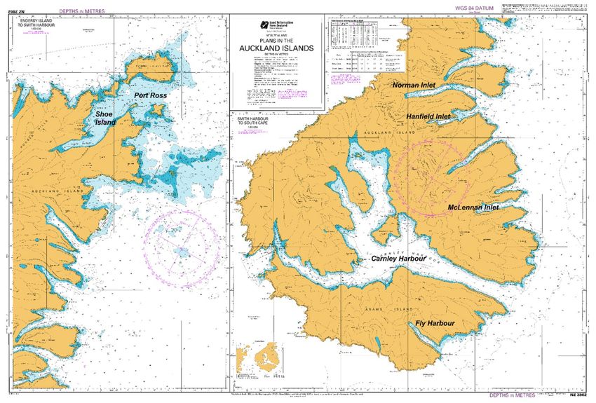
Geosciences 2019, 9, 56                                                                             2 of 17

specifications for data gathered for nautical charts. Licensed mariners and most commercial operators
are legally required to keep their charts and nautical publications up to date [4].
     In contrast to charts, seafloor terrain and habitat maps are created to represent the entirety of the
seafloor at the highest resolution possible, are not subject to legal or standardized requirements for
data collection, processing, or presentation, and are intended for a variety of uses. Seafloor maps can
identify areas characterized by sediment type, show locations suited to particular species or highlight
areas requiring protection, demonstrate benefits to areas that are receiving protection, and identify
change over time [5–7]. As a result, these maps are characterized by much more variability than charts.
Knowledge of the epoch represented by map data can be crucial for studies considering oceanographic
and geologic processes from tidal cycles to millennia. Similarly, data resolution and measurement
uncertainties vary and may affect how the map can or should be used. Derived geomorphic
attributes, such as depth, slope, and rugosity, which aid map creation and use [8], are also subject
to these limitations. Seafloor map design and scale depends on the scientific objectives of the
user [9], for example, large scale descriptive geomorphic modeling [10,11] or higher-resolution benthic
analysis [12].
     Today, all data used to create a chart is collected and archived digitally. As we look backward in
time, different components of a project will have been collected and stored in discrete packages [13].
For example, singlebeam echosounder traces recorded on paper are annotated with handwritten or
digitally stamped fix numbers. Fix numbers allowed the user to find the corresponding position,
logged in a fieldbook or computer data file. Working with such legacy data today may require
scanning the paper records and geolocation of the data, possibly involving interpolation between fixes.
Legacy data are not necessarily uniformly sampled. For example, the repetition rate of positioning
from sextant and theodolite observations proceeds at a different rate than that of echosounding.
Raw ancillary data, such as grab sampling, may only be preserved as written field observations while
today the digital record, including photographs, would be archived together with other data.
     This case study in the sub-Antarctic Auckland Islands, New Zealand (Figure 1) includes both
recent and legacy hydrographic data collected primarily for charting. Collecting and processing
high-quality, high-resolution bathymetric data used to generate marine habitat maps requires expert
knowledge and is time consuming, thus it is expensive. The isolation and inhospitable climate of
the Auckland Islands exacerbates these issues, but the area is of interest for environment and climate
research [14–17]. Our interest in the data is scientific—seabed morphology in the eastern fjords and
shelf records past glacier activity on the islands [18].
     Our case study may be particularly useful to researchers who do not have access to state-of-the-art
equipment, such as multibeam echosounders (multibeam hereafter), or as a reconnaissance tool for
those intending to work in areas that have not been recently surveyed due to factors, such as isolation
and associated field costs. It is timely as governments and hydrographic offices worldwide consider
the high cost of gathering data for their charts and look for ways to ensure these high-quality data
sources are of maximum benefit to secondary users [19].
Geosciences 2019, 9, 56                                                                            3 of 17

                                   Figure 1. Auckland Islands location.

2. Background
      In New Zealand, charting responsibility is held by Land Information New Zealand (LINZ),
who contract the collection of the underlying hydrographic data to commercial surveyors. A risk-based
approach is used to prioritize survey operations, which are shared in the long-term national
hydrographic survey plan, HYPLAN [1].
      Hydrographic data collected in New Zealand waters for the purposes of updating nautical charts
is held by LINZ and largely accessible online via the ‘LINZ Data Service’ (https://data.linz.govt.nz/).
Up-to-date georeferenced navigational charts as well as their individual components, such as sounding
points and contours, may be downloaded. Metadata includes elements, such as the date and design
scale of use, and points users to other documentation, which will allow appropriate and informed
use of the data. In the case of a chart, these will provide detailed information on the collection and
processing methods used to generate the chart (e.g., hydrographic standards and specifications for
nautical charts and publications) as well as how to interpret the symbols and abbreviations used.
LINZ direct mariners to NP5011 (INT1) Symbols and Abbreviations used on Admiralty Charts [20]. All data
is licensed for reuse under Creative Commons BY 4.0 NZ [21].
      Older data is often identified through the shapefile of an area, allowing the user to approach LINZ
to request copies of items, such as scanned hand-drawn airsheets containing depths and contours
from singlebeam echosounder (singlebeam hereafter) tracks, field reports, and multibeam surfaces.
Prior to 1996, the Royal New Zealand Navy (RNZN) had charting responsibility for New Zealand
waters. Raw data from that era is not held by LINZ [22].
      Users should be aware of the specific attributes of hydrographic charts, which may differ from
maps created for other purposes.

1.    Charted depths are referenced to Chart Datum (CD) (approximately Lowest Astronomical Tide
      (LAT)) while heights are above Mean High Water Springs (MHWS) [23,24]. Maps created for other
      purposes may use Mean Sea Level (MSL), ellipsoidal heights (when using Global Navigation
Geosciences 2019, 9, 56                                                                             4 of 17

      Satellite System (GNSS)), or a self-generated reference, and, in our experience, published seafloor
      maps often fail to specify any datum at all. Offsets between datums will be large in areas with
      large tidal ranges. Depths on products prior to chart publication—such as fairsheets—are usually
      on a Sounding Datum (SD) derived by the field surveyor. It may or may not be the same as
      CD [23,24].
2.    Depths indicated on charts are shoal biased. Processing of depth data preserves shallow areas,
      with very shallow points designated to ensure they are maintained through any processing,
      binning, surface, or contour creation [13,25,26].
3.    The precision of depths indicated on charts is standardized. In New Zealand, LINZ requires
      one decimal place display for depths of 0.1–30.9m (e.g., 5.68 becomes 5.6), and integer values
      for depths greater than 31m. Drying heights are rounded up to the nearest decimeter [23,24].
      Depth data collected for charts may be manually cleaned, filtered, or processed with algorithms,
      such as the Combined Uncertainty Bathymetric Estimator (CUBE) [23–27].
4.    Because of the legal and risk management implications of charted data, all field measurements are
      well calibrated with horizontal and vertical uncertainties quantified and field checks undertaken.
      Hydrographers collecting data for nautical charts will meet IHO s-44 standards as a minimum [28].
      In New Zealand, LINZ has refined these in their Contract Specifications for Hydrographic Surveys
      (HYSPEC) [23,24], which provides a useful guide for users of New Zealand chart data as readers
      will see every element of data collection laid out.

     Datum, processing and calibrations, checks, and uncertainty information are always recorded in
chart metadata and reports [13,23,24,26,29], though this may not exist for older legacy data [30]. This is
essential information for anyone trying to learn as much from a chart as possible, or synthesize chart
data with their own.
     While in the field, hydrographers collect ancillary information that will aid the mariner.
Examples of this include bottom samples taken to provide information for safe anchoring, tide,
and current observations. Here too, chart data is biased toward the concerns of the mariner, for example,
bottom samples tend to be collected at potential anchorages. In our case study on the Auckland
Islands, the ancillary data includes magnetic anomalies and areas of particularly dense kelp [26,29,31].
Grain size classifications from bottom samples can be used for initial benthic mapping and tide
and current information can extend a habitat map to consider the ocean conditions associated with
a particular habitat type. Daily logs, weather reports, and final report observations may also be helpful
for planning new fieldwork, especially in remote locations, such as our case study.
     The Auckland Islands (Maungahuka in the Māori language) are an isolated island group in the
Southern Ocean. At around 51◦ S 166◦ E they are about 400 km south of mainland New Zealand.
They are part of the New Zealand Sub-Antarctic Islands United Nations Educational Scientific and
Cultural Organization (UNESCO) World Heritage Site [32]. The islands show terrestrial and submarine
evidence of Quaternary glaciation [14–18]. Interest in the island group is growing, with increasingly
frequent visits by cruise vessels, conservation, fishing, and military patrol ships. Prior to post-2015,
nautical charts around the Auckland Islands were compiled from depth information collected between
1840 and 1991, the latter undertaken with singlebeam by the RNZN along the eastern shelf and into
some eastern inlets [29,33]. Other inlets had no depth information. In recognition of the growing
vessel traffic, conservation risks and other concerns LINZ contracted hydrographic survey firm,
iX Survey (now iXblue), to undertake a multibeam survey of the entire eastern side of the island in
2015. This provided near complete bathymetric coverage of an area 660 km2 (c.f. terrestrial island area
of 568 km2 ) and was the first time some inlets had been charted [26,31].

3. Materials and Methods
     We analyzed and compared legacy 1991 singlebeam (referred to here as pre-2015) and
recently-collected multibeam (referred to here as post-2015) bathymetric data, in combination with
Geosciences 2019, 9, 56                                                                                            5 of 17

ancillary chart information in an investigation of the seafloor of the Auckland Islands (Table 1).
The ‘Chart Data Collection Date’ is obtained from the Source Data diagram on the charts. Fairsheets and
sheet images are the official bathymetric product created by the hydrographer. They show selected
soundings in a grid-like fashion over the survey area, along with contours and points of interest.
Until recently, charts were always created from these sheets and spatially uniform depth uncertainty
could be reported. Now, the high-density data collected by modern multibeam is characterized by
spatially variable measurement uncertainty, and statistically derived surfaces are more commonly
used [34].

                            Table 1. Legacy chart data used in the Auckland Islands case study.

                                                                 Chart Data Collection        Published Chart
                          Item                 Data Source
                                                                  Dates (Surveyors)            Edition Date
                 Pre-2015 survey
                 Chart NZ2862                    LDS 1                 1840–1991 2                  2005
               Fairsheet 2862-25 3            LDS request 1          1991 (RNZN 4 )                 1991
                 Report HI 158                LINZ request            1991 (RNZN)                   1991
                 Post-2015 survey
            Chart NZ2862 (Figure 2)               LDS 1                 1980–2015                   2017
         Processed bathymetric surface         LINZ request      2015 (iXSurvey/LINZ)               2015
         Sheet Image HS42-STD-07-v2 3          LINZ request      2015 (iXSurvey/LINZ)               2015
         Sheet Image HS42-STD-06-v2 3          LINZ request      2015 (iXSurvey/LINZ)               2015
                 Report HS42                   LINZ request      2015 (IXSurvey/LINZ)               2015
      1 LINZ Data Service (https://data.linz.govt.nz/); 2 1840-1945 “Sketch surveys from various sources”, 1980–1991

      “HMNZS Monowai”; 3 Norman and Hanfield Inlets; 4 Royal New Zealand Navy.

      Figure 2. Annotated chart NZ2862, 2017 edition © LINZ (Downloaded from LINZ Data Service
      (https://data.linz.govt.nz/).

      Multibeam sounders can also collect backscatter data and this may be used for habitat
analysis [35,36]. Collection, but no processing, was specified by LINZ in post-2015 and the data
currently only exist as raw files [26]. As minimal specifications existed during its collection, this data
is likely to face similar issues to those experienced by Dolan et al. [19]. Those authors found large
backscatter variations when contracted hydrographers focused solely on bathymetry collection on the
Geosciences 2019, 9, 56                                                                            6 of 17

Norwegian shelf. Backscatter is not considered here. Starting in 2016, backscatter requirements have
been instituted in New Zealand [23].
     Reports HI 158 and HS42 were consulted and information that would aid either analysis of the
existing survey data, or support those planning to visit the area in the future, were compiled.
     The pre-2015 fairsheet 2862-25 was sent with a group of .tiff files covering the entire RNZN survey
area, all of which required georeferencing. Processed multibeam data from the post-2015 Auckland
Islands survey was provided by LINZ in CARIS HIPS and SIPS (Hydrographic Information Processing
System and Sonar Information Processing System) proprietary CSAR (Caris Spatial Archive) format at
1m grid note spacing. This was exported as a raster GeoTIFF.
     Processing steps followed in ArcMap v10.3.1. were:

5.    Visual analysis: Georeferenced charts, multibeam geotiff, and fairsheets were all imported for
      initial examination of data and display attributes. This included identification of changes between
      charted epochs, comparison of differences between the chart products and other depth data,
      and consideration of the vertical datums of each.
6.    Bathymetric analysis: Here, we focus on Norman and Hanfield Inlets, an area of geologic
      interest [14, 18] covered by chart data from both epochs. Depths from fairsheet 2862-25 were
      digitized manually in ArcMap at the centroid of each value posting. Contours were digitized as
      polylines following the fairsheet contour. Location errors are estimated to be ±3.5 m and ±2.5 m,
      respectively, using the line widths and resolution of map elements. Both were processed with the
      ArcMap Spline with Barriers function at 3 m (the sonar footprint given at a depth of 10 m in Report
      HI 158) to create a depth raster. Slope (for each cell), ruggedness (Vector Ruggedness Measure
      (VRM) in neighborhood of 5), and aspect (downslope direction of maximum date of change in
      each cell) were calculated using the Benthic Terrain Modeler (BTM) v.3 [37] for both epochs.
7.    Ancillary data: Bottom sample and other chart data were digitized from the two versions
      of NZ2862 with the modern sample records checked against those in Report HS42.
      Sample characteristics from the charts and reports were classified for rendering as a habitat
      map using the following: Rock, gravel, pebbles, coral, shells, broken shells, coarse sand, sand,
      fine sand, and mud, with samples described using multiple classes given an average value.
      The resulting data were gridded using an Inverse Distance Weighting (IDW) function and a 100 m
      cell size.

4. Results
    The 1991 and 2015 Reports of Survey on the singlebeam and multibeam surveys, respectively,
contain descriptive and technical components of use to scientists. The key elements of use to support
analysis or planning for future voyages are described in Table 2.
Geosciences 2019, 9, 56 7 of 17
Table 2. Auckland Islands survey report information.
Item Pre-2015 [29] Post-2015 [26]
For data analysis
Time period of field survey 5–25 February 1991 14 January–28 March 2015
Topography and texture descriptive section.
Topography and texture descriptive section. 4 inlets Multibeam survey over 660 km2 survey area
Completion of survey areas complete, Norman and Musgrave for small craft including northern and eastern inlets and Carnley
navigation only. Approaches on shelf only. Harbour, and section of eastern shelf. Singlebeam
data collected at heads of some bays.
Geodetic control Transverse Mercator WGS 72, Auckland Island Grid. WGS84, UTM 58S
Trisponder and GPS interface. Some theodolite Wide Area Differential GNSS (WADGNSS)
Positioning
transits used in steep areas. Marinestar G2 and HP solutions
4x tide stations installed. SD recovered from
1x tide station. SD transferred from Bluff.
Tides and Sounding Datum previous work.Co-tidal model used. ADCP tide
Logship tide stream observations.
stream observations.
Atlas Deso 20 singlebeam: 33 and 210 kHz. Konsberg 2040C multibeam swath at 4–6x water
Bathymetry 3 m footprint in 10 m depth. Lines perpendicular depth. Attitude and calibrations detailed.
to contours. Odom/Atlas singlebeam.
Shipek grab sampler, photographed, none retained.
Sampling Dredge, none retained. At heads of inlets and locations suitable for
anchoring. 5 km spacing offshore.
From aerial photo NZMS 270 From LINZ provided satellite imagery at
Coastline
1036/2. (260 series is 1:50,000) 0.6 m resolution.
Calibrations All calibrations listed. All calibrations listed and detailed in other reports.
For future work
Planning considered this would be extreme,
Forecast valuable—rapid changes. Difficult to
but conditions were generally favorable with only
Weather conditions establish terrestrial survey network in low cloud and
3 days of 73 lost to weather downtime.
boggy peat.
Calmer offshore in the mornings.
Surveyors consulted high-resolution satellite images
as part of their field planning. Kelp (Durvillaea
Thick “Bull Kelp” growing “on all shoals of 20 m or
Antarctica) “ . . . thick and often impenetrable” up to
Bathymetry less” caused echosounder multipath and
100 m off coast prevented measurements. Large swell
access difficulties.
created dangerous conditions beside the coast in
exposed areas.
High water anomaly referred to in NP51 NZ Surveyed through kelp at mid-tide when patches
Tides
Pilot observed. were “tow(ed) under”.
Safety considerations - all parties equipped for
Many coastline photos. Methods for working in kelp
Other observations 3 days solo in field no matter how short task
areas discussed.
duration. Suitable landing sites listed.
To compare epochs, we must be certain about the vertical datum used at each stage of the charting
process. In our case, we consulted with LINZ and confirmed the SD in post-2015 was equal to CD [38].
The same should be true for the pre-2015 data as indicated in the report (Table 2). That is, that the
pre-2015 control locations are stable and recoverable. Without this information in the post-2015 report
we would need some other means to co-reference the datasets, perhaps by selecting several permanent
seabed features (e.g., large rocky areas) and holding the depths of these fixed. Additional information
would be required in seismically active areas where there may be relative motion over short distances.
4.1. Visual Analysis
The most recent version of chart NZ2862 “Plans in the Auckland Islands” is shown in Figure 2.
The most important change from the pre-2015 chart is depths added in previously uncharted inlets
and bays, North Harbour, Matheson Bay, Webling and Haskell Bay, Chambres, Granger, Griffith, Deep,
Worth, and McLennan Inlets in the north and east, and in Carnley Harbour, Bollons Bay, and Fly
Harbour to the south. Significant new detail has also been added in Port Ross and around the easterly
islands and reefs. Plans for additional seabed mapping or other scientific investigations could be made
using either of these charts.
The implications of the new data are considerable detail for Norman, Hanfield, and McLennan
Inlets and Fly Habour (Figure 2). Sills are major geomorphic features in the fjords and while an
older version of the chart shows sills in Norman and Hanfield inlets, Fly and McLennan were not
surveyed at that time. Text on both epochs of the chart report a local magnetic anomaly at Shoe Island
in Port Ross and point users to the Notes. The 2005 version states “Shoe Island is reported to be
highly magnetic”, while 2017 comments “A local magnetic anomaly is reported to exist in the areaGeosciences 2019, 9, 56 8 of 17
indicated on this chart”. This is likely related to the volcanic origins of the island group [39] (Figure 2).
Interestingly, the post-2015 chart (Figures 2 and 3b) includes far less detail than its predecessor.
Figure 3. Norman and Hanfield Inlet study area: (a) Chart NZ2862 2005 edition, location of the
isolated low discussed in the text is circled in purple; (b) Chart NZ2862 2017 edition; (c) pre-2015
fairsheet2862-25, “R” symbol discussed in the text is circled in green; (d) post-2015 Standard sheets
HS42-STD-06&07; (e) Bathymetric surface created from (c), prominent seabed features discussed in the
text are circled in blue; (f) Bathymetric surface from .csar file with 0 values interpolated to coastline
contour in (d).
The pre-2015 fairsheet and post-2015 standard sheet both contain more information than what
is displayed on the charts. The shape of the shoreline is more detailed in 2015. Pre-2015 coastline
was taken from aerial photo enlargement and checked with optical instruments. Post-2015 coastline
was delineated from high-resolution satellite imagery and checked with GNSS observations (Table 2).
Numerous kelp beds are shown on the pre-2015 fairsheets (Figure 6d), fewer are shown on the
post-2015 standard sheets, and even fewer appear on the charts (Figures 3a and 6d). Instead, kelp bed
locations on the chart are more often shown as shallow areas and reef symbols. The digital rendering of
depths on the post-2015 sheet image is less orderly than the hand-drafted pre-2015 fairsheet (Figure 3d).
The fairsheet from pre-2015 contains information about shoreline features, composition of beaches,
and annotated notes while the standard sheet from post-2015 has fewer observational notes.
4.2. Bathymetric Analysis
Derived products, such as shaded relief images, and maps of bed slope and other quantities can
be generated using the legacy fairsheet data (Figure 3c). The 1991 fairsheet depths, spaced ~75 m apart,
were interpolated to a 3 m grid for this purpose. After noting the use of singlebeam at the heads of
some bays mentioned in the post-2015 survey (Table 2), care was taken to confirm that this did not
apply in either Norman or Hanfield Inlets. Thus, the post-2015 shaded relief surface (Figure 3f) does
not have any additional equipment varying uncertainties or resolutions that should to be taken into
account. The different error characteristics of the pre- and post-2015 data must be examined in theirGeosciences 2019, 9, 56 9 of 17
own right before derived products are compared quantitatively, for example, differencing surfaces
for change detection; see, for example, [30,40]. Nevertheless, qualitative comparison of the two
data sets (Figure 3e,f) reveals some interesting differences—and motivations to return to the legacy
fairsheet data.
Finer resolution hydrographic data does not necessarily yield more scientifically useful data in
the final nautical chart. For example, the older chart (Figure 3a) indicates more detail on the Norman
Inlet sill. The features are relatively smoother on the more recent chart (Figure 3b) and it barely shows
remnants of retreat moraines along the shorelines, inland of the main sill. The sills are evidence of past
glacier extent and these features likely impounded terrestrial lakes when the sea level was lower than
at present [15,18]. Consulting only the more recent chart when planning new fieldwork or inferring
details of past glaciation could thus be misleading.
Resolution of the hydrographic data does of course influence elevation model creation. While the
same shoaling features are apparent in both the pre- and post-2015 surfaces (Figure 3e,f), regridding the
sparse 1991 measurements appears to have created unrealistic undulations and isolated lows in regions
that are very smooth in the post-2015 surface. One particularly notable example, an isolated low in
Norman Inlet indicated by a purple circle in Figure 3, corresponds to a very deep sounding, 57 m on
the pre-2015 fairsheet (Figure 3c). The local low was captured within the 50 m contour and is thus
invisible to the pre-2015 chart (Figure 3a). The shoal bias inherent in charting makes this seabed feature
of little interest for that purpose. It only becomes apparent when the pre-2015 fairsheet is consulted.
Depth bias in charting also appears in the Hanfield Inlet basin. The pre-2015 chart shows a deepest
point of 53 m, while the deepest post-2015 charted value is 48 m. The pre-2015 fairsheet (Figure 3c)
shows a depth of 53 m in this area, while the post-2015 surface (Figure 3f) is 54.7 m. There has been
little change in the underlying data, but the chart has changed considerably.
All the concerns discussed above are apparent in the difference map created by subtracting the
surface created by digitized pre-2015 fairsheet from the post-2015 surface (Figure 4). A grid-like pattern
of alternating positive and negative differences in flat areas is due to different grid spacings of two
datasets. Echo sounding records the shoalest point within the beam footprint. Multibeam sounding
footprints are smaller than singlebeam, thus they more precisely represent the seabed within each
footprint along the swath. With the use of GNSS positioning, the horizontal location of this shoalest
point is similarly more precise [13]. This effect is evident in the negative differences along the fiord
walls (Figure 4a). The post-2015 multibeam survey better represents their steep slopes than does the
pre-2015 survey. The positive differences along the coastline are due to the wider multibeam swath,
which measures much further beyond the nadir region of the vessel.Geosciences 2019, 9, 56 10 of 17
Figure 4. Norman and Hanfield Inlet differencing: (a) Difference between post-2015 multibeam surface
and pre-2015 fairsheet surface, note buff color is −0.7 m; (b) histogram of differences with 1 m bins;
(c&d) areas of rock outcrops used for shoal analysis with pre-2015 fairsheet overlaid.
A blunder involving vertical datum would generate a systematic offset between the two datasets.
Following our suggestion above, we compared depths on two prominent seabed features (blue circles
in Figures 3e and 4), rocky areas that we assume to be persistent across epochs. We focused on the
difference in the shoalest depth on each feature because this is a specific focus of data collection for
charting. Rather than an offset, we found +1.2 m and −1.1 m differences (Figure 4c,d ). The legacy
data are too coarse to allow the distributions of the differences to be compared. It is also important
to recognize that due to equipment limitations, the pre-2015 survey may not have actually found the
shoalest point despite careful investigation of the area. Examining larger or more features might clarify
the source of the offset, but our interpretation is that it is due to better representation of fiord wall
slopes in the post-2015 survey.
Morphologic attributes of the sea floor are more well-resolved by the higher resolution multibeam
data, but this may be more important for some attributes than others (Figure 5). In our case study,
the slope result is similar for both (Figure 5a,b), while some details of aspect and ruggedness appear to
be missing in the pre-2015 data set. The overall sense of relatively rougher and smoother areas is the
same in both data sets, while the higher-resolution multibeam surveys captured more detail than the
older singlebeam surveys.Geosciences 2019, 9, 56 11 of 17
Figure 5. Bathymetric surface outputs for the Norman and Hanfield Inlet study area created
using Benthic Terrain Modeler (BTM) v.3.0 in ArcMap 10.3.1 [37]: (a) Pre-2015 slope; (b) post-2015
slope; (c) pre-2015 terrain ruggedness; (d) post-2015 terrain ruggedness; (e) pre-2015 aspect;
(f) post-2015 aspect.
4.3. Ancillary Information
Bottom sample classifications were interpolated to make sediment type maps for easy visualization
(Figure 6). The gradients do not represent transitions in sediment type, rather, changes in the color
maps represent changes in knowledge of the sediment type. Our post-2015 map incorporates both pre-
and post-2015 data. The main difference between the two is additional spatial detail and an improved
knowledge of the seabed materials in Carnley Harbor and offshore, thanks to samples collected in
2015. In most cases, the additional samples confirm the earlier classifications. This is encouraging as
common practice is for sediment size to be determined by visual inspection only and thus be somewhat
subjective. The heads of all inlets surveyed are mud or fine sand and the sills where samples have
been collected tend to be characterized by coarser sediments. The “R”, rocky seabed, identification
may represent either a seabed sample or denote the location of a shoal feature where the mariner is
advised to take care.
It should not be assumed that the more recent chart represents the more complete or correct
ancillary data. While samples add spatial detail in Norman and Hanfield Inlets (Figure 5d,e),
some ancillary information about rocks (“R” in Figure 3a,c ), shoreline conditions, and kelp beds
(light green diamonds in Figure 6d) has been removed from the post-2015 charts. This change could
represent improved knowledge, a change in cartographic standards, or a change in the physical
environment. In one example, an “R” near the head of Hanfield Inlet shown in the pre-2015 chart
and fairsheet is not present in the post-2015 versions. Considering the physical setting—proximity to
steep cliffs and a waterfall (see also Figure 6 in [18])—rockfall debris is likely to accumulate along the
shoreline. We conclude that omitting the ancillary information is a cartographic choice. All available
charts and ancillary data should be considered when using and interpreting both new and legacy
data sets.Geosciences 2019, 9, 56 12 of 17
Figure 6. Bottom samples and chart symbols translated into sediment-type maps: (a) Surface from
bottom samples from pre-2015 chart NZ2862 (2005); (b) surface from bottom samples from post-2015
chart NZ2862 (2017); (c) Norman and Hanfield Inlet surface from bottom samples from chart NZ2862
2005 edition, with location of plotted kelp symbols (green diamonds); (d) Norman and Hanfield Inlet
surface from bottom samples from chart NZ2862 2017 edition.
5. Discussion
In some respects, the bathymetric elements of this case study are a simple demonstration of the
ability of modern equipment to improve data capture. However, we also demonstrate that older
legacy data is useful, especially when paired with the other ancillary information available on charts.
The closing paragraph of the iX Survey report expresses the hope of the hydrographer that the new
charts will enable future research and conservation activities to happen safely in the Auckland Islands
area [26].
The use of existing data during reconnaissance is expected. Indeed, legacy data supports campaign
length calculations in terms of swath coverage, and allows speed/coverage/density tradeoffs to be
considered as realistically as possible. We suggest here that other uses are also valuable. While legacy
data products may appear at first glance to be sparser than more modern data, when examined
comprehensively (such as on a fieldsheet) they may provide a more detailed view of the seabed
than anticipated.
Care must be taken to understand the limitations inherent in nautical charts. Comparison between
charted data and hydrographic fieldsheets or surfaces in Figure 3 demonstrates the wealth of
information not presented to the target audience of nautical charts (the mariner concerned with
safe navigation). A nautical chart has an uneven spacing of contours—typically at 5, 10, 20, 30, 50,
and 100 m—such that features of interest to geomorphic and habitat studies and campaign planning
may be obscured. The reduction in chart data discussed in Section 4.1 seen in the number of soundings
labelled, terrestrial contours, and smoothing of the bathymetric contours serves a purpose—the
nautical cartographer must be confident that what is displayed is all that is needed by the mariner.
In the interest of making our case, we have given several examples of interesting features that mightGeosciences 2019, 9, 56 13 of 17
not be recognized using only the most recent nautical charts in our study area. However, other features
would not have been anticipated at all, for example, the shoaling and partial sills identified in Deep,
Chambres, Granger, Waterfall Inlets, and Carnley Harbour using the post-2015 surface [18].
Derived bathymetric products all reflect the resolution of the underlying data, although we found
that general characteristics were similar across the pre- and post-2015 data sets. Depending on the
intended application of derived products, high-cost, higher resolution data may not substantially
change the result of any given analysis. From the point of view of planning, areas characterized by
shorter or longer wavelength variability and thus of interest for particular types of field campaigns
would be similarly identified using either data set.
The analysis of seabed sediment type is useful, but limited by several factors. Firstly, the samples
are described qualitatively by (well-meaning) hydrographers. In our case study, “gravel” was identified
several times in the pre-2015 survey, while the term “pebble” was used in the post-2015 survey.
Both terms can be used for grain sizes ranging from 4 to 64 mm, but such details are not explained in the
survey reports. Survey specifications requiring photographs of the seabed, sieving, sample retention,
or coding aligned with the SEDCLASS, the U.S. Geological Survey ArcMap Sediment Classification
Tool [41], would address this issue. Additionally, the locations of seabed samples are biased toward
anchorages in our pre-2015 case [29], unless a specific request has been made, for example, along the
perimeter of the survey area, in our post-2015 example [26]. There is neither the sampling density nor
a protocol that might be expected for a full geological mapping survey.
Other information on a chart may support geological and biological investigations. For example,
kelp beds (Figure 6d) only grow on rocky or stony substrates. This information may go unrecognized
if only the nautical chart is consulted. By utilizing the fairsheet data along with plotting other rock
symbols (submerged, awash, drying), users of legacy chart data (and potentially other products,
such as high-resolution satellite images) may find that much of the hard substrate in the survey
area can be said to be ‘known’ to some extent, so efforts can focus in the softer, smoother sediment.
As multispectral backscatter research indicates it is of most use in these finer sediment areas [42],
this initial reconnaissance can be used as a quick tool to focus modern technologies to places they will
be most effective.
Should chart data be synthesized in our seafloor maps? We have demonstrated some benefits of
this additional data, but it is important to consult the hydrographic survey reports and consider the
challenges we have also identified, including shoal bias, truncated precision, and clarity regarding SD
or CD referenced depths. In [18], we used tidal and geodetic observations to ascertain the CD to MSL
offset for the area to link our map with terrestrial observations.
Once datum issues are resolved it is very useful that the data are collected to recognized
standards, calibrated thoroughly, and the means to analyze the measurement uncertainty exists.
Previous calculations of the vertical uncertainty associated with the data in the Auckland Islands puts
the post-2015 multibeam depths at ±0.4 m to ±1.6 m @ 95% Cl (using MB-1 specs [18,24]) and the
older data at ±0.5 m to ±3.3 m at 95% Cl (assuming IHO Order 1 inshore and Order 3 offshore) [18,28].
Calibrations and uncertainty considerations are the strength of hydrographic measurements, and while
older equipment may have meant researchers undertaking seafloor mapping fieldwork did not
see the effects of poorly calibrated data, this is no longer the case with the high-precision rapid
data collecting gear used today. Lecours et al. and Lucieer et al. [43–45] demonstrate the effect of
motion sensor calibration issues on data derivatives and advocate for more consideration of this by
researchersusing digital terrains in seafloor mapping. Synthesis of hydrographic calibration, checks,
metadata, and reporting methods from nautical charting into general seafloor mapping would be of
great benefit to the marine scientific community today and for users of our data in the future. This is
recognized in [46]. Quantitative change detection via differencing datasets from different epochs is
a primary motivation of work, like ours [30,42,47]. In this case study, differences appear to be associated
with methods of data collection and processing rather than environmental change. The mean difference
we calculated, -0.6m (Figure 4b) lies within the range of total propagated vertical uncertainty, ±0.6 mGeosciences 2019, 9, 56 14 of 17
to ±3.7 m at 95% Cl. Another approach to detect change and investigate measurement uncertainties
would be to down-sample the raw post-2015 multibeam data at the locations of the pre-2015 singlebeam
depth points and compare the two. This approach could be particularly useful with more widely
spaced legacy data.
The samples on the chart could be integrated into seafloor mapping classifications.
Interpretation challenges may arise when details are removed in a chart update without explanation.
In our case study, does the removal of the “R” indicating a rocky seabed mean the annotation on
the pre-2015 chart was incorrect, or that rock that was there in pre-2015 is no longer present in
post-2015, indicating change over time in this environment? In our experience conducting nautical
charting surveys, one rule-of-thumb was to classify a site with three or more unsuccessful grabs as “R”.
Thus, even if the designation is removed on cartographic grounds (such as relevance to the intended
user), there may be other reasons to exercise caution. In the case study presented here, we examined
the surrounding terrestrial features and concluded that rockfall was likely in at least one location
where an ”R” had been removed. If such seabed features were important to our study, we would have
a clear reason to visit such sites, but only because we compared the new and old charts and sheets.
We recognize that in New Zealand, we benefit from an all-of-government open data environment
that enabled us to free and open access of the data used in this case study. Other studies incorporating
legacy data have obtained it from, for example, British Admiralty Charts [40], United Stations National
Ocean Service (NOS) and the National Oceanic and Atmospheric Administration (NOAA) [30,48],
and the Hydrographic Service of the Royal Netherlands Navy [47]. While we did not have access
to the raw data from 1991 through LINZ, researchers in other countries may have access to scans of
archived analog recordings, for example, the NOAA Marine Geophysical Trackline Data documented
by the National Geophysical Data Centre [48,49]. An additional benefit of access to analogue records is
that signal intensity could be analyzed for applications, like acoustic ground discrimination for habitat
classification, and could be applied to the legacy data. [7].
6. Conclusions
This short case study reveals the important primary and ancillary data that exist behind the
nautical charts commonly consulted for seabed mapping voyage planning or during data analysis.
Charts and ancillary data from surveys in pre-2015 and post-2015 are shown to provide useful seafloor
information in the Auckland Islands. The addition of the primary data (fairsheets and surfaces) greatly
improves the bathymetric analyses able to be undertaken. Improvements can be made to seabed
sampling specifications for nautical charting to support a wider variety of users and those users would
benefit from understanding the existing charting specifications so that they can correctly use existing
data, or indeed ensure their data is useful to others in the future.
Author Contributions: E.J.T. developed the idea, processed the data, analyzed the results and prepared the
manuscript including all figures and tables. C.L.H. advised on the approach and analysis and co-wrote
the manuscript.
Funding: This research received no external funding.
Acknowledgments: The authors thank two anonymous reviewers both for their interest in the work and
suggestions that improved the manuscript. We thank A. Price and Land Information New Zealand (LINZ)
for assistance with the multibeam bathymetric data. Analyses were undertaken using academic licenses for CARIS
HIPS&SIPS 9.0 and Arc GIS 10.3.1. Figures created must not be used for navigation. Hydrographic data in this
paper are held by Land Information New Zealand (LINZ), and are licensed for reuse under CC BY 4.0 (contact:
customersupport@linz.govt.nz).
Conflicts of Interest: The authors declare no conflict of interest.
References
1. Land Information New Zealand (LINZ). New Zealand Hydrographic Authority HYPLAN; Land Information
New Zealand: Wellington, New Zealand, 2017.Geosciences 2019, 9, 56 15 of 17
2. Maritime & Coastguard Agency U.K. SOLAS Guidance on Chapter V—Safety of Navigation.
Available online: http://solasv.mcga.gov.uk/ (accessed on 28 December 2018).
3. International Hydrographic Organization (IHO). Regulations of the IHO for International (IHO) Charts and Chart
Specifications of the IHO; International Hydrographic Organization: Principauté de Monaco, Monaco, 2018.
4. Land Information New Zealand (LINZ). Applying Corrections to Charts and Nautical Publications.
Available online: https://www.linz.govt.nz/sea/maritime-safety/notices-mariners/about-notices-
mariners/applying-corrections-charts-and-nautical-publications (accessed on 28 December 2018).
5. Zakariya, R.; Azhafiz Abdullah, M.; Che Hasan, R.; Khalil, I. The Use of Backscatter Classification and
Bathymetry Derivatives from Multibeam Data for Seabed Sediment Characterization. In Engineering
Applications for New Materials and Technologies; Advanced Structured Materials; Öchsner, A., Ed.; Springer:
Cham, Switzerland, 2018; Volume 85, pp. 579–591.
6. Boswarva, K.; Butters, A.; Fox, C.J.; Howe, J.A.; Narayanaswamy, B. Improving marine habitat mapping
using high-resolution acoustic data; a predictive habitat map for the Firth of Lorn, Scotland. Cont. Shelf Res.
2018, 168, 39–47. [CrossRef]
7. Brown, C.J.; Smith, S.J.; Lawton, P.; Anderson, J.T. Benthic habitat mapping: A review of progress towards
improved understanding of the spatial ecology of the seafloor using acoustic techniques. Estuar. Coast.
Shelf Sci. 2011, 92, 502–520. [CrossRef]
8. Micallef, A.; Le Bas, T.P.; Huvenne, V.A.I.; Blondel, P.; Hühnerbach, V.; Deidun, A. A multi-method approach
for benthic habitat mapping of shallow coastal areas with high-resolution multibeam data. Cont. Shelf Res.
2012, 39–40, 14–26. [CrossRef]
9. Lecours, V.; Devillers, R.; Schneider, D.; Lucieer, V.; Brown, C.; Edinger, E. Spatial scale and geographic
context in benthic habitat mapping: Review and future directions. Mar. Ecol. Prog. Ser. 2015, 535, 259–284.
[CrossRef]
10. Heap, A.D.; Harris, P.T. Geomorphology of the Australian margin and adjacent seafloor. Aust. J. Earth Sci.
2008, 55, 555–585. [CrossRef]
11. Porskamp, P.; Rattray, A.; Young, M.; Ierodiaconou, D. Multiscale and hierarchical classification for benthic
habitat mapping. Geosciences 2018, 8, 119. [CrossRef]
12. Che Hasan, R.; Ierodiaconou, D.; Laurenson, L.; Schimel, A. Integrating Multibeam Backscatter Angular
Response, Mosaic and Bathymetry Data for Benthic Habitat Mapping. PloS ONE 2014, 9. [CrossRef]
[PubMed]
13. Calder, B. On the Uncertainty of Archive Hydrographic Data Sets. IEEE J. Ocean. Eng. 2006, 31. [CrossRef]
14. Browne, I.M.; Moy, C.M.; Riesselman, C.R.; Neil, H.L.; Curtin, L.G.; Gorman, A.R.; Wilson, G.S. Late
Holocene intensification of the westerly winds at the subantarctic Auckland Islands (51◦ S), New Zealand.
Clim. Past Discuss. 2017, 1–37. [CrossRef]
15. Hodgson, D.A.; Graham, A.G.C.; Roberts, S.J.; Bentley, M.J.; Cofaigh, C.Ó.; Verleyen, E.; Vyverman, W.;
Jomelli, V.; Favier, V.; Brunstein, D.; et al. Terrestrial and submarine evidence for the extent and timing of the
Last Glacial Maximum and the onset of deglaciation on the maritime-Antarctic and sub-Antarctic islands.
Quat. Sci. Rev. 2014, 100, 137–158. [CrossRef]
16. McGlone, M.S. The Late Quaternary peat, vegetation and climate history of the Southern Oceanic Islands of
New Zealand. Quat. Sci. Rev. 2002, 21, 683–707. [CrossRef]
17. Rainsley, E.; Turney, C.S.M.; Golledge, N.R.; Wilmshurst, J.M.; McGlone, M.S.; Hogg, A.G.; Li, B.;
Thomas, Z.A.; Roberts, R.; Jones, R.T.; et al. Pleistocene glacial history of the New Zealand subantarctic
islands. Clim. Past Discuss. 2018, 1–50. [CrossRef]
18. Tidey, E.; Hulbe, C. Bathymetry and glacial geomorphology in the sub-Antarctic Auckland Islands.
Antarct. Sci. 2018. [CrossRef]
19. Dolan, M.; Thorsnes, T.; Chand, S.; Bjarnadóttir, L.R.; Ofstad, A.E.; Tappel, Ø. Towards Multibeam Data
Acquisition Specifications which Promote Good Backscatter Data: Experiences from the MAREANO
Programme, Norway. In Proceedings of the GEOhab 2018, Santa Barbara, CA, USA, 7–11 May 2018.
20. Admiralty Publication. NP5011 Symbols and Abbreviations Used on Admiralty Charts, 7th ed.; United Kingdom
Hydrographic Office: Taunton, UK, 2018.
21. Land Information New Zealand (LINZ). LINZ Data Service. Land Information New Zealand, CC BY 4.0 NZ.
Available online: https://data.linz.govt.nz/ (accessed on 15 January 2018).
22. Caie, S.; (Land Information New Zealand, LINZ). Personal communication, 2019.Geosciences 2019, 9, 56 16 of 17
23. Land Information New Zealand (LINZ). Contract Specifications for Hydrographic Surveys, Version 1.3, New Zealand
Hydrographic Authority; Land Information New Zealand: Wellington, New Zealand, 2016; pp. 1–95.
24. Land Information New Zealand (LINZ). Contract Specifications for Hydrographic Surveys, Version 1.2,
New Zealand Hydrographic Authority; Land Information New Zealand: Wellington, New Zealand, 2010.
25. De Oliveira Junior, A.M.; Jeck, I.K. Multibeam Processing for Nautical Charts (Using CUBE and
“Surface Filter” to enhance multibeam processing. Int. Hydrogr. Rev. 2009, 2, 63–73.
26. IXSURVEY Australia Pty Ltd. Auckland Islands Hydrographic Survey—Report of Survey. Project Number:
HYD-2014/15-01 (HS42). Contract Number: HYD 1415-HS42; IXSURVEY Australia Pty Ltd.:
Wellington, New Zealand, 2015.
27. Calder, B.R.; Mayer, L.A. Automatic processing of high-rate, high-density multibeam echosounder data.
Geochem. Geophys. Geosyst. 2003, 4. [CrossRef]
28. International Hydrographic Organization (IHO). IHO Standards for Hydrographic Surveys; Special Publication
No 44; International Hydrographic Bureau: Principauté de Monaco, Monaco, 2008.
29. Hydrographic Office RNZN. Report of Survey HI 158. Inlets of the East Coast of Auckland Island;
Hydrographic Office RNZN, Hydrographic Office RNZN: Takapuna, Auckland, New Zealand, 1991.
30. Mitchell, N.C. Channelled erosion through a marine dump site of dredge spoils at the mouth of the Puyallup
River, Washington State. Mar. Geol. 2005, 220, 131–151. [CrossRef]
31. Land Information New Zealand (LINZ). NZ2862 Plans in the Auckland Islands. 2017. Available online:
http://www.linz.govt.nz/sea/charts/paper-charts/nz202-chart-catalogue/2862 (accessed on 15 January 2018).
32. United Nations Educational Scientific and Cultural Organization (UNESCO). Convention Concerning the
Protection of the World Cultural and Natural Heritage; UNESCO: Paris, France, 1998; p. 135.
33. Hydrographic Office RNZN. NZ2862 Plans in the Auckland Islands. 2005. Available online: http://www.
linz.govt.nz/sea/charts/paper-charts/nz202-chart-catalogue/2862 (accessed on 31 January 2014).
34. Hare, R.; Calder, B.; Alexander, L.; Sebastian, S. Multi-beam Error Management: New data processing trends
in hydrography. Hydro Int. 2008, 8, 6–9.
35. Brown, C.J.; Blondel, P. Developments in the application of multibeam sonar backscatter for seafloor
habitat mapping. Appl. Acoust. 2009, 70, 1242–1247. [CrossRef]
36. Lamarche, G.; Lurton, X. Recommendations for improved and coherent acquisition and processing of
backscatter data from seafloor-mapping sonars. Mar. Geophys. Res. 2017. [CrossRef]
37. Walbridge, S.; Slocum, N.; Pobuda, M.; Wright, D.J. Unified Geomorphological Analysis Workflows with
Benthic Terrain Modele. Geosciences 2018, 8. [CrossRef]
38. Price, A.; (Land Information New Zealand, LINZ). Personal communication, 2017.
39. Quilty, P.G. Origin and evolution of the sub-Antarctic islands the foundation. Pap. Proc. R. Soc. Tasman.
2007, 141, 35–58. [CrossRef]
40. Watts, A.B.; Nomikou, P.; Moore, J.D.P.; Parks, M.M.; Alexandri, M. Historical bathymetric charts and the
evolution of Santorini submarine volcano, Greece. Geochem. Geophys. Geosyst. 2015, 16, 847–569. [CrossRef]
41. O’Malley, J.U.S. Geological Survey ArcMap Sediment Classification Tool: Installation and User Guide U.S.
Department of the Interior; U.S. Geological Survey: Reston, VA, USA, 2007; p. 38.
42. Gaida, T.C.; Afrizal Tengku Ali, T.; Snellen, M.; Amiri-Simkooei, A.; van Dijk, T.A.G.P.; Simons, D.G.
A Multispectral Bayesian Classification Method for Increased Acoustic Discrimination of Seabed Sediments
Using Multi-Frequency Multibeam Backscatter Data. Geosciences 2018, 8. [CrossRef]
43. Lecours, V.; Devillers, R.; Edinger, E.N.; Brown, C.J.; Lucieer, V.L. Influence of artefacts in marine digital
terrain models on habitat maps and species distribution models: A multiscale assessment. Remote Sens.
Ecol. Conserv. 2017. [CrossRef]
44. Lecours, V.; Devillers, R.; Lucieer, V.L.; Brown, C.J. Artefacts in Marine Digital Terrain Models: A Multiscale Analysis
of Their Impact on the Derivation of Terrain Attributes. IEEE Trans. Geosci. Remote Sens. 2017, 55, 5391–5406.
[CrossRef]
45. Lucieer, V.; Huang, Z.; Siwabessy, J. Analyzing Uncertainty in Multibeam Bathymetric Data and the Impact
on Derived Seafloor Attributes. Mar. Geod. 2015, 39, 32–52. [CrossRef]
46. Lecours, V.; Dolan, M.J.; Micallef, A.; Lucieer, V.L. A review of marine geomorphometry, the quantitative
study of the seafloor. Hydrol. Earth Syst. Sci. 2016, 20, 3207–3244. [CrossRef]
47. Dorst, L.L. Survey Plan Improvement by Detecting Sea Floor Dynamics in Archived Echo Sounder Surveys.
Int. Hydrogr. Rev. (New Ser.) 2004, 5, 49–63.Geosciences 2019, 9, 56 17 of 17
48. Becker, J.J.; Sandwell, D.T.; Smith, W.H.F.; Braud, J.; Binder, B.; Depner, J.; Fabre, D.; Factor, J.; Ingalls, S.;
Kim, S.-H.; et al. Global Bathymetry and Elevation Data at 30 Arc Seconds Resolution: SRTM30_PLUS.
Mar. Geod. 2009, 32, 355–371. [CrossRef]
49. National Oceanic and Atmospheric Administration National Geophysical Data Centre (NOAA NGDC).
Marine Geophysical Trackline Data. Available online: http://www.ngdc.noaa.gov/mgg/geodas/geodas.html
(accessed on 12 January 2019).
© 2019 by the authors. Licensee MDPI, Basel, Switzerland. This article is an open access
article distributed under the terms and conditions of the Creative Commons Attribution
(CC BY) license (http://creativecommons.org/licenses/by/4.0/).You can also read