Simulation of a Severe Sand and Dust Storm Event in March 2021 in Northern China: Dust Emission Schemes Comparison and the Role of Gusty Wind - MDPI
←
→
Page content transcription
If your browser does not render page correctly, please read the page content below
atmosphere

Article
Simulation of a Severe Sand and Dust Storm Event in March
2021 in Northern China: Dust Emission Schemes Comparison
and the Role of Gusty Wind
Jikang Wang *, Bihui Zhang, Hengde Zhang, Cong Hua, Linchang An and Hailin Gui *

                                          National Meteorological Center, China Meteorological Administration, Beijing 100081, China;
                                          zhangbh@cma.gov.cn (B.Z.); zhanghd@cma.gov.cn (H.Z.); huacong@cma.gov.cn (C.H.); anlch@cma.gov.cn (L.A.)
                                          * Correspondence: wangjk@cma.gov.cn (J.W.); guihl@cma.gov.cn (H.G.)

                                          Abstract: Northern China experienced a severe sand and dust storm (SDS) on 14/15 March 2021. It
                                          was difficult to simulate this severe SDS event accurately. This study compared the performances
                                          of three dust-emission schemes on simulating PM10 concentration during this SDS event by imple-
                                          menting three vertical dust flux parameterizations in the Comprehensive Air-Quality Model with
                                          Extensions (CAMx) model. Additionally, a statistical gusty-wind model was implemented in the dust-
                                          emission scheme, and it was used to quantify the gusty-wind contribution to dust emissions and peak
                                          PM10 concentration. As a result, the LS scheme (Lu and Shao 1999) produced the minimum errors for
                                          peak PM10 concentrations, the MB scheme (Marticorena and Bergametti 1995) underestimated the
                                          PM10 concentrations by 70–90%, and the KOK scheme (Kok et al. 2014) overestimated PM10 concen-
                                          trations by 10–50% in most areas. The gusty-wind model could reasonably reproduce the probability
                                          density function of 2-min wind speeds. There were 5–40% more dust-emission flux and 5–40% more

                                   peak PM10 concentrations generated by the gusty wind than the hourly wind in the dust-source
Citation: Wang, J.; Zhang, B.; Zhang,     regions. The increase of peak PM10 concentration caused by gusty wind in the non-dust-source
H.; Hua, C.; An, L.; Gui, H.              regions was higher than in the dust-source regions, with 10–50%. Implementing the gusty-wind
Simulation of a Severe Sand and Dust      model could help improve the LS scheme’s performance in simulating PM10 concentrations of this
Storm Event in March 2021 in              severe SDS event. More work is still needed to investigate the reliability of the gusty-wind model
Northern China: Dust Emission             and LS scheme on various SDS events.
Schemes Comparison and the Role of
Gusty Wind. Atmosphere 2022, 13, 108.     Keywords: sand and dust storms; gusty-wind model; vertical dust flux parameterizations; CAMx
https://doi.org/10.3390/
atmos13010108

Academic Editor: Thomas Gill
                                          1. Introduction
Received: 10 December 2021
Accepted: 8 January 2022
                                                Sand and dust storms (SDSs) are extremely hazardous weather systems characterized
Published: 10 January 2022                by low visibility, strong wind, and high particle-matter concentration that frequently occur
                                          in arid and semi-arid regions such as East Asia [1–3]. There were about ten SDSs events per
Publisher’s Note: MDPI stays neutral
                                          year in East Asia in the last 20 years, and the variations of the frequency and intensity SDSs
with regard to jurisdictional claims in
                                          events were closely related to surface conditions and the intensity of the polar vortex [2,4].
published maps and institutional affil-
                                          SDSs events not only cause loss of life and agriculture destruction but also influence weather
iations.
                                          and climate by disturbing radiation balance [1,5–7]. SDSs were shown to be an important
                                          source of PM10 pollution in East Asia [8,9]. Many methods, including observations and
                                          numerical models, have been used to comprehend SDSs processes [7,10–14].
Copyright: © 2022 by the authors.               Studies have been performed to improve the model performance on the simulation of
Licensee MDPI, Basel, Switzerland.        SDS events. Parameterization of dust-emission flux is one of the main challenges in dust-
This article is an open access article    model development [10]. Several dust-emission schemes have been developed to estimate
distributed under the terms and           dust emission. These dust-emission schemes can reasonably well simulate the SDSs events.
conditions of the Creative Commons        However, the dust emissions vary by several orders of magnitude when using different
Attribution (CC BY) license (https://     dust-emission schemes [10,15–17]. Kang et al. [15] reported that the vertical dust fluxes
creativecommons.org/licenses/by/          differed greatly under the same horizontal dust flux condition because the sandblasting
4.0/).

Atmosphere 2022, 13, 108. https://doi.org/10.3390/atmos13010108                                       https://www.mdpi.com/journal/atmosphere
Atmosphere 2022, 13, 108                                                                                          2 of 14

                           efficiency varied among these dust-emission schemes. Other studies also indicated that
                           sandblasting efficiency was crucial for simulating dust-emission fluxes [16,17].
                                 Gusty wind also plays an important role in modeling the dust-emission flux. The
                           large variations in gusty-wind speed and the coherent structure of gusty wind could
                           generate more dust-emission flux than the steady wind [18,19]. Wang and Zheng [20]
                           predicted the sand-transport rates, respectively, under steady and unsteady wind, using
                           a one-dimension model. Results showed that the sand-transport rates by unsteady wind
                           could be 10–200% higher than the steady wind [20]. However, the gusty wind was neglected
                           and simplified as the hourly wind in most dust-emission schemes [11]. Studies about gusty-
                           wind parameterization [21–23] and the probability density function of gusty wind [24]
                           made it possible to consider the gusty wind in dust-emission schemes.
                                 Northern China experienced a severe SDS in March 2021, leading to excessive particu-
                           late pollution and strong wind [25–27]. Yin et al. [26] analyzed the climatological causes
                           of this SDS event. They concluded that the strong gusty wind in the dust-source area
                           corresponded to the increases in the PM10 concentration in Beijing, China. This study
                           implements three vertical dust-flux parameterizations in the Comprehensive Air-Quality
                           Model with Extensions (CAMx) to investigate their performances on this severe SDS event.
                           A gusty-wind prediction model was developed to simulate the probability density function
                           of gusty-wind speed and implemented in the dust-emission scheme to quantify the role of
                           gusty wind in this SDS event. Atmospheric rivers intertwined strongly with exceptional
                           SDS events [28,29]; hence, we also analyzed the possible influence of atmospheric rivers on
                           this exceptional SDS event.

                           2. Data and Methods
                           2.1. Data
                                The weather phenomena, 10 m wind speed, 2 m temperature, visibility, and PM10
                           concentrations were obtained from China Meteorological Administration. Two-minute
                           average 10 m wind speed and max instantaneous 10 m wind speed were used to analyze
                           the probability density function of gusty wind in Northern China. The instantaneous wind
                           speed was a 3 s—sample wind speed. Hourly PM10 concentrations in six sites, including
                           three sites near the dust-source regions and three sites in the transport pathway, were used
                           to test the model performance on dust emission and transportation. PM10 concentrations
                           over 6500 µg/m3 were recorded as 6500 µg/m3 , due to the limitation of measurements in
                           some stations, such as Hohhot and Yinchuan. The bias, root mean square error (RMSE),
                           and the index of agreement (IOA), which were explained in detail in Baker et al. [30], were
                           used to evaluate the simulation of wind and PM10 concentrations. Moderate-resolution
                           imaging spectroradiometer (MODIS) aerosol optical depth (AOD) data, at 550 nm from the
                           Deep Blue algorithm over land, was also used to evaluate the simulated AOD.

                           2.2. Model Configuration
                                 The Comprehensive Air-Quality Model with Extensions (CAMx) was used to model
                           the transport and diffusion of particle matters [31]. The CAMx model was an off-line chem-
                           istry transport model. The Weather Research and Forecasting model (WRF 4.0) [32] was
                           used to generate meteorological fields for CAMx and the dust-emission model. The first
                           24 h were disregarded as spin-up for each SDSs episode modeling. Boundary and initial
                           conditions were derived from the National Centers for Environmental Prediction (NCEP)
                           final (FNL) global reanalysis data, with the resolution of 1◦ . The physical parameterization
                           options chosen for the WRF modeling included Dudhia shortwave radiation, RRTM long-
                           wave scheme, YSU planetary-boundary layer scheme, and the Unified Noah land-surface
                           scheme. The model domain covers most of East Asia. The model has a horizontal grid
                           spacing of 24 km, with 30 vertical levels from the surface to 50 hpa. Figure 1 shows the
                           model domain.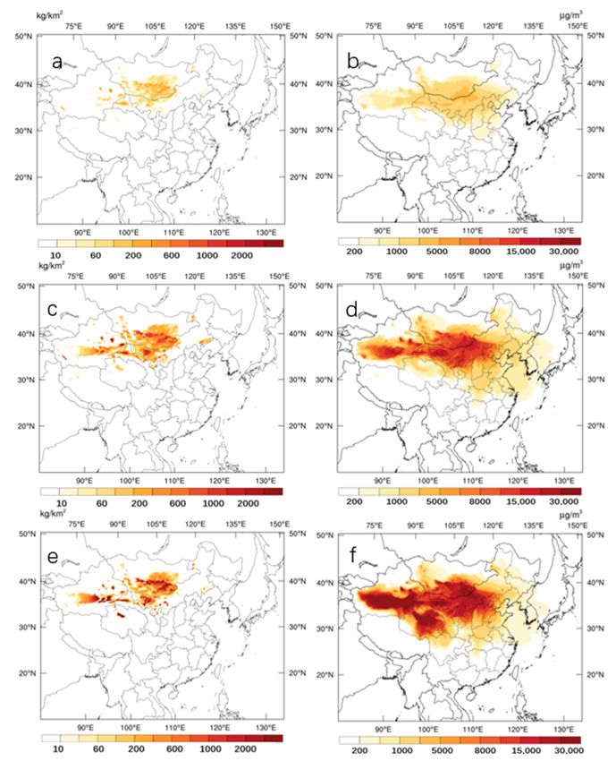
Atmosphere 2022, 13, 108                                                                                                                3 of 14

                           Figure 1. Model domain and the PM10 monitoring stations (the black dots) used to evaluate the model.

                           2.3. Dust-Emission Schemes
                                A dust-emission scheme was used to generate windblown dust emissions for CAMx,
                           based on a revised approach used in the global ECHAM/MESSy atmospheric chemistry–
                           climate model [33,34]. The scheme calculates dust-emission flux based on surface friction
                           velocity and threshold surface friction–velocity. The threshold friction-velocity depends on
                           the size of soil particles, air density, and soil moisture, which was explained in detail in
                           our previous study [9]. Three vertical dust-emission parameterizations were implemented
                           in the dust-emission scheme to perform an inter-comparison of different dust-emission
                           parameterizations.
                                The first vertical dust-flux parameterization (MB scheme) was proposed by Marti-
                           corena and Bergametti [35]. The relationship between vertical and horizontal dust fluxes is
                           related to the clay content of soils less than 20%.

                                                         F = 100 × Q × 100.134 f c −6.0 ( f c < 20)                                        (1)

                           where F is the vertical dust emission flux, Q is the horizontal dust flux, and f c is the clay
                           content in %.
                                 The second vertical dust-flux parameterization (LS scheme) was proposed by Lu and
                           Shao [5]. In the LS scheme, the saltation bombardment efficiency ratio F/Q is linearly
                           proportional to the fraction of dust contained in the soil and inversely proportional to the
                           soil surface-hardness parameter.
                                                                                       r
                                                             Cα g f s ρb                 ρp
                                                       F=                  0.24 + Cβ u∗     Q                          (2)
                                                                2p                       p

                           where Cα and Cβ are constant values; g is the gravitational acceleration; p is the plastic
                           pressure of soil surface in N/m2 ; f s is the sand fraction in soil; ρb and ρ p are the bulk-soil
                           and soil-particle density, respectively; and u∗ is surface friction velocity. The bulk-soil
                           density in our model refers to Liu et al. [25], and other parameters in the LS scheme refer to
                           Kang et al. [15].
                                The third vertical dust-flux parameterization (KOK scheme) was defined in the study
                           of Kok et al. [11]. In the KOK scheme, soil erodibility is a critical parameter for calculating
                           dust-emission flux.
                                                                                                                      Cα u∗st −u∗st0
                                                                                          ρ a u2∗ − u2∗t

                                                               u∗st −u∗st0
                                                        (−Ce      u∗st0    )                                    u∗            u∗st0
                                            F = Cd0 e                          f bare f c                                                  (3)
                                                                                               u∗st             u∗t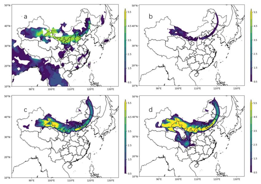
Atmosphere 2022, 13, 108                                                                                                 4 of 14

                           where Cd0 , Ce , and Cα are dimensionless coefficients; ρ a is the air density; u∗t is the threshold
                           friction velocity; u∗st is the standardized threshold friction velocity, which is defined as the
                           value of u∗t at standard atmospheric density at sea level (1.225 kg/m3 ); u∗st0 is standardized
                           threshold friction velocity for the highly erodible soil, which is set to 0.16 m/s; and f bare is
                           the fraction of the surface that consists of bare, erodible soil. The parameters setting refers
                           to the study of Kok et al. [11].
                                 The land cover, land-surface information, and dust size distribution in the model
                           can be found in our previous study [9]. We implement these three schemes in the CAMx
                           wind-blowing dust scheme to simulate the SDSs.

                           2.4. Gusty Wind Scheme
                                 A statistical model for predicting wind-speed probabilities [24] was used to char-
                           acterize the gusty wind during the SDS episode. Efthimiou et al. [24] reported that the
                           statistical behavior of near-surface wind speeds could be adequately represented by the
                           Beta distribution, which was even slightly better than the widely used Weibull distribution.
                           The probability density function (PDF) for the time-averaged horizontal wind speed is
                           given as follows:
                                                                                         ηα−1
                                                                      V α −1

                                                            V                        V
                                                    pd f          ∝             1−                                  (4)
                                                           Vmax     Vmax            Vmax
                                                                      1 η
                                                                 α=           −1                                    (5)
                                                                    1+η I
                                                                           Vmax − Va
                                                                    η=                                                      (6)
                                                                              Va
                                                                              σV2
                                                                        I=                                                  (7)
                                                                             Va 2
                           where V is the wind speed, Vmax is the max wind speed over a period of time, Va is the
                           mean wind speed over a period of time, I is the wind speed fluctuation intensity, and σV2 is
                           variance of wind speed.
                                According to Harper et al. [36] and Suomi et al. [37], the standard deviation of the
                           wind speed can be estimated as follows:

                                                                           Vmax − Va
                                                                    σV =                                                    (8)
                                                                              aσ

                                A simple parameterization is used to parameterize Vmax [38] as follows:

                                                                      Vmax = bg Va                                          (9)

                           where aσ and bg are the two factors (normalized gust wind speed and gust factor) for pre-
                           dicting the standard deviation of wind speed and max wind speed by using the mean wind
                           speed. These two factors can be obtained from the statistics of the observed wind speed.
                                The processes mentioned above allow us to use the WRF output hourly wind speed
                           and the statistical factors to parameterize the distribution of gusts. We implement this
                           gusty-wind model in the dust-emission scheme to quantify the contribution of gusty wind
                           to dust-emission flux.

                           3. Results and Discussion
                           3.1. Sand and Dust Storm Event Description
                                In Mongolia and Northern China, a super-strong Mongolian cyclone
                           (min SLP = 978 hPa, Figure 2a) triggered a severe SDS event on 14/15 March 2021 [26].
                           The minimum visibility was much lower than 0.5 km, and the wind speed exceeded 15 m/s
                           in Mongolia and Northwestern China during this SDS episode (Figure 2c). The sand dust
                           particles were transported to most areas to the north of the Yangtze River by the north
Atmosphere 2022, 13, 108                                                                                                  5 of 14

                           wind and caused low visibility (
Atmosphere 2022, 13, 108 6 of 14
Figure 3. Distribution of max instantaneous wind speed (a) and statistical factors of gusty wind
during the period from 13 to 15 March 2021. (b) Ratio of hourly max instantaneous to hourly max
2-min wind speed, (c) the normalized gust wind speed (Equation (8)) of 2-min wind speed, (d) the
correlation coefficient of the standard deviation (σV ) with the difference between the max and the
mean 2-min wind speed in 1-h period, (e) the gust factor (Equation (9)) of 2-min wind speed, and (f)
the correlation coefficient of the max with the mean 2-min wind speed in 1-h period.
We used the 2-min averaged wind speed to calculate the standard deviation and max
wind speed over a 1-h period. The normalized gusty-wind speeds (defined in Equation (8))
ranged from 2.3 to 2.7 at most stations over Northern China (Figure 3c). In other words, the
gust-wind speeds tended to be about 2.5 standard deviations away from the average wind
speed. The correlation coefficients of the standard deviation (σV ) with the difference be-
tween the max and the mean 2-min wind speed were around 0.9 (Figure 3d), which lent high
confidence in estimating the standard deviation by using normalized gust-wind speeds.
The gust factor is another parameter for the gusty-wind model. The max 2-min wind
speed can be estimated by Equation (9). The gust factor ranged from 1.2 to 1.3 for stations
in Inner Mongolia (Figure 3e). The correlation coefficients were greater than 0.9 (Figure 3f)
between hourly max 2-min wind speed and hourly mean wind speed. The max 2-min wind
speed could be used to estimate the standard deviation. However, it could not be used in
Equation (6) to estimate the wind PDF, because the max 2-min wind speed was a measured
value, rather than an extreme value as a direct consequence of statistical uncertainties
associated with limited measuring times [24]. Therefore, we used the max instantaneous
wind speed to approximate the extreme wind speed in Equation (6). The max instantaneous
wind can also be estimated by Equation (9) by replacing the mean wind speed with the
max 2-min wind speed. The hourly max instantaneous to hourly max 2-min wind speed
ratio ranged from 1.4 to 1.6 in most stations (Figure 3b).
In this study, aσ was set to be 2.5, and the gust factor was set as 1.25 for the max
wind speed in Equation (8) and 1.5 × 1.25 for max wind speed in Equation (6). In order to
evaluate the gusty-wind model scheme, the frequency of measured 2-min wind speed atAtmosphere 2022, 13, 108 7 of 14
an hourly average wind speed of 10 m/s was used to verify the model. The gusty wind
could reproduce the PDF of 2-min wind speed (Figure 4). As shown in Table 1, the WRF
model performance on the wind was satisfied and comparable with results from other
studies [30]. The model slightly overestimated the wind speeds in dust-source regions.
Generally, jointing of gusty-wind model and WRF model could reasonably estimate the
PDF of wind speed.
Figure 4. Probability density function (PDF) of measured 2-min wind speed (solid line) and PDF
generated by the gusty-wind model (dash line) at an hourly average wind speed of 10 m/s.
Table 1. Statistic parameters of WRF model performance on wind and temperature during 14–15
March 2021 (Northwest China, including Xinjiang, Gansu, Ningxia, Shaanxi, and Inner Mongolia in
China; Northern China, including Beijing, Hebei, Shanxi, Shandong, and Henan in China).
Wind Speed Wind Direction Temperature
BIAS (m/s) RMSE (m/s) IOA BIAS (◦ ) BIAS (K) RMSE (K) IOA
Mongolia 0.48 1.78 0.7 −4.8 −1.11 1.67 0.93
Northwest China 0.96 1.17 0.87 6.3 −1.54 2.56 0.95
Northern China 0.69 1.62 0.85 7.2 −1.43 2.84 0.87
3.3. Comparison of the Simulated PM10 Concentrations Generated by the Three Schemes
Three abovementioned vertical dust-emission parameterizations were used to simulate
the SDS episode. Figure 5 showed the distributions of total dust-emission flux and the
peak PM10 concentrations during the SDS episode simulated by the three schemes. The
MB scheme generated the lowest dust emission flux and PM10 concentration, and the
KOK scheme generated the highest. The dust-emission flux and peak PM10 concentration
generated by the LS scheme were about 6–10 times and 3–6 times than by the MB scheme,
respectively. The distribution of peak PM10 concentration, using the LS scheme, was similar
to the distribution of visibility (Figure 2c). The peak PM10 concentration was higher than
5000 µg/m3 in the area where the min visibility was lower than 1 km and was higher than
200 µg/m3 in the area where the min visibility was lower than 7.5 km. The KOK scheme
generated much higher PM10 concentrations, especially in Qinghai, where the min visibility
was about 4 km. The MB scheme generated much lower PM10 concentrations, especially in
the Taklimakan desert, where the min visibility was lower than 1 km.Atmosphere 2022, 13, 108 8 of 14
Figure 5. Simulated total dust-emission flux (kg/km2 , (a,c,e)) and the peak PM10 concentrations
(µg/m3 , (b,d,f)) during the sand and dust episode using three dust-emission schemes ((a,b), using
MB scheme; (c,d), using LS scheme; (e,f), using KOK scheme).
PM10 concentrations in six sites were used to evaluate the performance of the three
schemes (Figure 6 and Table 2). Three sites (Hohhot, Yinchuan, and Lanzhou) were located
near the dust-source areas. The peak PM10 concentrations exceeded 6500 µg/m3 in Hohhot
and Yinchuan. The LS and KOK schemes reproduced high PM10 concentrations, but the
MB scheme underestimated PM10 concentrations. The LS scheme produced the minimum
error for the peak PM10 concentrations in Lanzhou, with about −609 µg/m3 . PM10 concen-Atmosphere 2022, 13, 108 9 of 14
trations in Beijing, Zhengzhou, and Jinan were used to evaluate dust transportation. The
MB scheme underestimated the peak PM10 concentrations at all three sites by large margins,
about 70–90%. The LS scheme produced the minimum errors for peak PM10 concentrations,
and the KOK scheme overestimated the peak PM10 concentrations at all three sites. The
IOA was around 0.9 for the three schemes in four sites, indicating the model could capture
the variation of PM10 concentration.
Figure 6. Comparison of simulated PM10 concentrations with observations (OBS: the observed PM10
concentrations, the concertation over 6500 µg/m3 was not recorded because of the limitation of
measurements in Hohhot and Yinchuan; MB, LS, and KOK were the simulated PM10 concentrations,
using MB, LS, and KOK schemes, respectively. Time is BJT).
Table 2. Statistic parameters of model performance on PM10 concentrations during SDS event.
(The IOA for Hohhot was not provided, because there were 12 missing values which exceeded
6500 µg/m3 ).
Peak PM10 (µg/m3 ) Mean PM10 (µg/m3 ) IOA
OBS MB LS KOK OBS MB LS KOK MB LS KOK
Beijing 7685 1239 7076 10,616 2698.9 432.0 2182.8 2787.8 0.97 0.97 0.94
Hohhot >6500 2599 12,036 25,394 >2793.7 573.9 2490.0 5073.5 / / /
Yinchuan >6500 2133 11,513 16,119 >2975.2 562.7 2867.3 5128.7 0.88 0.87 0.90
Lanzhou 4086 478 3488 6334 2934.9 221.7 1696.4 3110.0 0.69 0.71 0.53
Zhengzhou 1826 363 1682 2453 736.2 156.7 612.7 696.0 0.97 0.98 0.98
Jinan 3522 462 2796 4102 1097.4 148.8 844.2 1015.8 0.90 0.90 0.88Atmosphere 2022, 13, 108 10 of 14
The AOD values reached 4.5 over Northern China (Figure 7a) at 10:30 a.m. on 15
March 2021, and the southern boundary of the area with a high AOD value (>2.5) in
Southern Hebei and Central Shanxi. All three schemes could reproduce the distribution of
AOD over Northern China. Due to the lack of anthropogenic emissions, the model did not
generate the distribution of AOD in Southern Asia. The AOD values simulated by the three
schemes (Figure 7b–d) were as varied as the simulated PM10 concentrations. MB scheme
underestimated the AOD by a large margin, with the maximum value being only around 1.
The KOK scheme overestimated the AOD, with the highest value exceeding 6. The LS
scheme performed better on simulating AOD than the other two schemes. However, it still
underestimated the AOD in the area around Hetao plain and overestimated the AOD in
Northwest China.
Figure 7. MODIS observed AOD (a) and simulated AOD by the three schemes ((b) MB, (c) LS, and
(d) KOK) at 10:30 a.m. on 15 March 2021.
3.4. The Role of Gusty Wind
The gusty-wind model (Section 2.4) could reproduce the PDF of 2-min average wind,
which could be considered as gusty disturbances [41]. We used the PDF of 2-min average
wind to calculate the PDF friction velocity in one hour and then generated the dust-
emission flux.
Figure 8 shows the percentage changes of simulated dust-emission flux and max
PM10 concentration caused by implementing the gusty-wind model. In most parts of
the dust-source area, the gusty wind generated 5–40% more dust-emission flux than the
hourly averaged wind. In the edge area of the dust source, the value reached 200%. These
results were consistent with Wang and Zheng [20], where a one-dimensional numerical
model of unsteady sand saltation was used to quantify the effects of the unsteady wind on
sand-transport rate. Implementing the gusty-wind model could lead to a 5–40% increase in
the peak PM10 concentration in the dust-source area and a 10–50% increase in East–Central
China. Therefore, the gusty wind could generate greater dust-emission flux, and more dust
particles could be transported to downwind regions. The increase in PM10 concentration
was greater and more widespread than the increase in dust-emission flux. The gusty
model generated the biggest percentage increase in dust-emission flux and the peak PM10Atmosphere 2022, 13, 108 11 of 14
concentrations with the KOK scheme and the smallest with the MB scheme because the
vertical flux parameterization was not related to wind speed in the MB scheme.
Figure 8. Percentage changes of simulated dust-emission flux (a,c,e) and peak PM10 concentration
(b,d,f) caused by the implementation of gusty-wind model ((a,b) use MB scheme, (c,d) use LS scheme,
and (e,f) use KOK scheme).
In Section 3.3, the LS scheme performed better when simulating PM10 concentrations
than the other two schemes for this SDS episode. Implementing the gusty wind in the
LS scheme could improve the model’s performance in regard to simulating the PM10
concentrations (Table 3). In Section 3.3, the LS scheme underestimated the peak and the
mean PM10 concentrations. The model with the gusty-wind scheme reduced the modeling
biases for the peak and the mean PM10 concentrations. For instance, the error was reduced
from −6.7% to −1.4% for mean PM10 concentration in Beijing.Atmosphere 2022, 13, 108 12 of 14
Table 3. Simulation biases of peak PM10 and mean PM10 , using LS scheme (LS) and implementing
gusty-wind model (LS-GUST).
Bias (µg/m3 ) Schemes Beijing Lanzhou Zhengzhou Jinan
LS −609 (−7.9%) −598 (−14.6%) −144 (−7.8%) −726 (20.6%)
Peak PM10
LS-GUST 314 (4.1%) 169 (4.1%) 90 (4.9%) −347 (−9.8%)
LS −516.1 (−6.7%) −1238.5 (−30.3%) −123.4 (−6.7%) −330.0 (−9.3%)
Mean PM10
LS-GUST −110.2 (−1.4%) −814.4 (−19.9%) 22.9 (1.2%) −90.1 (−2.5%)
Note: PM10 concentrations at four sites which had no missing data were used to evaluate the model with
gusty-wind scheme.
Northern China experienced another SDS event on 27–29 March. This SDS event was
much weaker than the SDS event on 14 to 15 March, with lower peak PM10 concentra-
tions [25,27]. In order to investigate the reliability of the gusty-wind model with the LS
scheme, the same model configurations were used to simulate the SDS event on 27–29
March. The evaluation results (Table 4) indicated that the LS scheme generated the lowest
biases in most cities. However, the biases were much larger for the SDS event on 27–29
March than the SDS event on 14/15 March. The gusty-wind model with the LS scheme
overestimated the peak PM10 concentration by 10~154%. More work is needed to improve
model’s reliability on various SDS events.
Table 4. Simulated and observed peak PM10 concentrations during SDS event on 27/28 March 2021
(values in brackets are relative errors).
Peak PM10 (µg/m3 ) Beijing Hohhot Yinchuan Zhengzhou Jinan
Observed 3347 2968 3425 1395 1061
MB-GUST 1053 (−69%) 1284 (−57%) 977 (−71%) 345 (−75%) 534 (−50%)
LS-GUST 4419 (32%) 5500 (85%) 4206 (23%) 1529 (10%) 2698 (154%)
KOK-GUST 9058 (171%) 11,889 (301%) 6932 (102%) 2760 (98%) 5625 (430%)
4. Conclusions
Northern China experienced an exceptional SDS event triggered by a super-strong
Mongolian cyclone and loose land surfaces on 14/15 March 2021. There was an atmospheric
river that could enhance the intensity of the Mongolia cyclone through the latent heat
release. This study compared the performance of three vertical dust-flux parameterizations
on the severe sand and dust storm event during 14/15 March 2021 by implementing these
three schemes in the CAMx model. There was a tenfold difference between the dust-
emission flux generated by these three schemes, while the difference between the peak
PM10 concentrations was up to six times. The MB scheme [35] underestimated the PM10
concentrations by 70–90%, while the KOK scheme [11] overestimated PM10 concentrations
in most areas by 10–50%, especially for Qinghai. The LS scheme [5] produced the minimum
errors for peak PM10 concentrations.
A statistical gusty-wind model was implemented in the dust-emission model. The
gusty wind model could reasonably reproduce the probability density function of 2-min
wind speeds. In the dust-source regions, compared with the hourly wind, dust-emission
flux and peak PM10 concentrations generated by the gusty wind increased by 5–40%. The
percent increase of dust-emission flux due to gusty wind could reach 200% on the edge of
the dust-source area. The increase of peak PM10 concentration caused by gusty wind in
the non-dust-source region was higher than that in the dust-source region, with 10–50%.
Considering the underestimations of the LS scheme, implementing the gusty-wind model
could improve the LS scheme’s performance on PM10 concentration simulation for the
severe SDS event on 15 March 2021.
Our study was based on an extreme SDS event, and it was difficult to conclude that a
particular scheme was adaptable for modeling and forecasting SDSs in Northern China.
For instance, our model did not simulate the SDS event on 27 to 29 March as accurately as
it did for the SDS event on 14 to 15 March. More studies for various SDS events are neededAtmosphere 2022, 13, 108 13 of 14
to improve the model performance. The gusty-wind model only considers the variation of
wind speed. Therefore, further works are expected in developing the gusty-wind model to
consider the effects of the coherent structure of gusty wind.
Author Contributions: Conceptualization, methodology, software, validation, formal analysis, and
original draft preparation, J.W.; resources, L.A.; supervision, project administration, and funding
acquisition, B.Z., C.H. and H.G.; writing—review and editing, H.Z. All authors have read and agreed
to the published version of the manuscript.
Funding: This work was funded by the National Research Program for Key Issues in Air Pollution
Control (DQGG2021301), the National Natural Science Foundation of China (41905121), and China
Meteorological Administration (CXFZ2021J023).
Institutional Review Board Statement: Not applicable.
Informed Consent Statement: Not applicable.
Data Availability Statement: All data for this study are available from the corresponding author on
request.
Acknowledgments: We made some figures by using Meteorological Diagnostic Tools (MetDig,
https://github.com/nmcdev, accessed on 9 December 2021) developed by Yu Gong and Kan Dai
from National Meteorological Center of CMA.
Conflicts of Interest: The authors declare no conflict of interest.
References
1. Zhang, X.-Y.; Gong, S.L.; Zhao, T.L.; Arimoto, R.; Wang, Y.Q.; Zhou, Z.J. Sources of Asian dust and role of climate change versus
desertification in Asian dust emission. Geophys. Res. Lett. 2003, 30, 6–9. [CrossRef]
2. An, L.; Che, H.; Xue, M.; Zhang, T.; Wang, H.; Wang, Y.; Zhou, C.; Zhao, H.; Gui, K.; Zheng, Y.; et al. Temporal and spatial
variations in sand and dust storm events in East Asia from 2007 to 2016: Relationships with surface conditions and climate
change. Sci. Total Environ. 2018, 633, 452–462. [CrossRef] [PubMed]
3. Zhou, C.; Gui, H.; Hu, J.; Ke, H.; Wang, Y.; Zhang, X. Detection of New Dust Sources in Central/East Asia and Their Impact on
Simulations of a Severe Sand and Dust Storm. J. Geophys. Res. Atmos. 2019, 124, 10232–10247. [CrossRef]
4. Yao, W.; Gui, K.; Wang, Y.; Che, H.; Zhang, X. Identifying the dominant local factors of 2000–2019 changes in dust loading over
East Asia. Sci. Total Environ. 2021, 777, 146064. [CrossRef]
5. Lu, H.; Shao, Y. A new model for dust emission by saltation bombardment. J. Geophys. Res. Space Phys. 1999, 104, 16827–16842.
[CrossRef]
6. Sun, H.; Pan, Z.; Liu, X. Numerical simulation of spatial-temporal distribution of dust aerosol and its direct radiative effects on
East Asian climate. J. Geophys. Res. Earth Surf. 2012, 117. [CrossRef]
7. Shao, Y.; Dong, C.H. A review on East Asian dust storm climate, modelling and monitoring. Glob. Planet. Chang. 2006, 52, 1–22.
[CrossRef]
8. Guan, Q.; Luo, H.; Pan, N.; Zhao, R.; Yang, L.; Yang, Y.; Tian, J. Contribution of dust in northern China to PM10 concentrations
over the Hexi corridor. Sci. Total Environ. 2019, 660, 947–958. [CrossRef]
9. Wang, J.; Gui, H.; An, L.; Hua, C.; Zhang, T.; Zhang, B. Modeling for the source apportionments of PM10 during sand and dust
storms over East Asia in 2020. Atmos. Environ. 2021, 267, 118768. [CrossRef]
10. Shao, Y. Simplification of a dust emission scheme and comparison with data. J. Geophys. Res. Space Phys. 2004, 109. [CrossRef]
11. Kok, J.F.; Mahowald, N.M.; Fratini, G.; Gillies, J.A.; Ishizuka, M.; Leys, J.F.; Mikami, M.; Park, M.-S.; Park, S.-U.; Van Pelt, R.S.;
et al. An improved dust emission model—Part 1: Model description and comparison against measurements. Atmos. Chem. Phys.
Discuss. 2014, 14, 13023–13041. [CrossRef]
12. Ju, T.; Li, X.; Zhang, H.; Cai, X.; Song, Y. Parameterization of dust flux emitted by convective turbulent dust emission (CTDE) over
the Horqin Sandy Land area. Atmos. Environ. 2018, 187, 62–69. [CrossRef]
13. Cheng, X.; Zeng, Q.-C.; Hu, F. Characteristics of gusty wind disturbances and turbulent fluctuations in windy atmospheric
boundary layer behind cold fronts. J. Geophys. Res. Space Phys. 2011, 116. [CrossRef]
14. Yang, X.; Yang, F.; Zhou, C.; Mamtimin, A.; Huo, W.; He, Q. Improved parameterization for effect of soil moisture on threshold
friction velocity for saltation activity based on observations in the Taklimakan Desert. Geoderma 2020, 369, 114322. [CrossRef]
15. Kang, J.Y.; Yoon, S.C.; Shao, Y.; Kim, S.W. Comparison of vertical dust flux by implementing three dust emission schemes in
wrf/chem. J. Geophys. Res. Atmos. 2011, 116, D09202. [CrossRef]
16. Tian, R.; Ma, X.; Zhao, J. A revised mineral dust emission scheme in GEOS-Chem: Improvements in dust simulations over China.
Atmos. Chem. Phys. Discuss. 2021, 21, 4319–4337. [CrossRef]Atmosphere 2022, 13, 108 14 of 14
17. Ma, S.; Zhang, X.; Gao, C.; Tong, D.Q.; Xiu, A.; Wu, G.; Cao, X.; Huang, L.; Zhao, H.; Zhang, S.; et al. Multimodel simulations of a
springtime dust storm over northeastern China: Implications of an evaluation of four commonly used air quality models (CMAQ
v5.2.1, CAMx v6.50, CHIMERE v2017r4, and WRF-Chem v3.9.1). Geosci. Model Dev. 2019, 12, 4603–4625. [CrossRef]
18. Zeng, Q.; Cheng, X.; Hu, F.; Peng, Z. Gustiness and coherent structure of strong winds and their role in dust emission and
entrainment. Adv. Atmos. Sci. 2009, 27, 1. [CrossRef]
19. Cheng, X.; Zeng, Q.; Hu, F. Stochastic modeling the effect of wind gust on dust entrainment during sand storm. Chin. Sci. Bull.
2012, 57, 3595–3602. [CrossRef]
20. Wang, P.; Zheng, X. Saltation transport rate in unsteady wind variations. Eur. Phys. J. E 2014, 37, 1. [CrossRef]
21. Kurbatova, M.; Rubinstein, K.; Gubenko, I.; Kurbatov, G. Comparison of seven wind gust parameterizations over the European
part of Russia. Adv. Sci. Res. 2018, 15, 251–255. [CrossRef]
22. Stucki, P.; Dierer, S.; Welker, C.; Gómez-Navarro, J.J.; Raible, C.C.; Martius, O.; Brönnimann, S. Evaluation of downscaled wind
speeds and parameterised gusts for recent and historical windstorms in Switzerland. Tellus A Dyn. Meteorol. Oceanogr. 2016, 68.
[CrossRef]
23. Patlakas, P.; Drakaki, E.; Galanis, G.; Spyrou, C.; Kallos, G. Wind gust estimation by combining a numerical weather prediction
model and statistical post-processing. Energy Procedia 2017, 125, 190–198. [CrossRef]
24. Efthimiou, G.C.; Hertwig, D.; Andronopoulos, S.; Bartzis, J.G.; Coceal, O. A Statistical Model for the Prediction of Wind-Speed
Probabilities in the Atmospheric Surface Layer. Bound.-Layer Meteorol. 2016, 163, 179–201. [CrossRef]
25. Liu, S.; Xing, J.; Sahu, S.K.; Liu, X.; Liu, S.; Jiang, Y.; Zhang, H.; Li, S.; Ding, D.; Chang, X.; et al. Wind-blown dust and its impacts
on particulate matter pollution in Northern China: Current and future scenarios. Environ. Res. Lett. 2021, 16, 114041. [CrossRef]
26. Yin, Z.; Wan, Y.; Zhang, Y.; Wang, H. Why super sandstorm 2021 in North China. Natl. Sci. Rev. 2021. [CrossRef]
27. Gui, K.; Yao, W.; Che, H.; Zheng, Y.; Li, L.; Zhao, H.; Zhang, L.; Zhong, J.; Wang, Y.; Zhang, X. Two mega sand and dust storm
events over northern China in March 2021: Transport processes, historical ranking and meteoro-logical drivers. Atmos. Chem.
Phys. 2021. preprint. [CrossRef]
28. Francis, D.; Fonseca, R.; Nelli, N.; Bozkurt, D.; Picard, G.; Guan, B. Atmospheric rivers drive exceptional Saharan dust transport
towards Europe. Atmos. Res. 2021, 266, 105959. [CrossRef]
29. Voss, K.K.; Evan, A.T.; Ralph, F.M. Evaluating the Meteorological Conditions Associated with Dusty Atmospheric Rivers. J.
Geophys. Res. Atmos. 2021, 126, e2021JD035403. [CrossRef]
30. Baker, K.; Johnson, M.; King, S.; Ji, W. Meteorological Modeling Performance Summary for Application to PM2.5/Haze/Ozone
Modeling Projects. 2004. Available online: https://www.iowadnr.gov/portals/idnr/uploads/air/insidednr/regmodel/mm5
_mpe_dec2004.pdf (accessed on 9 December 2021).
31. Ramboll Environment and Health. User’s Guide, Comprehensive Air Quality Model with Extensions (CAMx), Version 7.00. 2020.
Available online: http://www.camx.com (accessed on 9 December 2021).
32. Skamarock, W.C.; Klemp, J.B.; Dudhia, J.; Gill, D.O.; Liu, Z.; Berner, J.; Wang, W.; Powers, J.G.; Duda, M.G.; Barker, D.M.; et al. A
Description of the Advanced Research WRF Version 4; NCAR Technical Note NCAR/TN-556+STR; National Center for Atmospheric
Research: Boulder, CO, USA, 2019; 145p. [CrossRef]
33. Klingmüller, K.; Metzger, S.; Abdelkader, M.; Karydis, V.A.; Stenchikov, G.L.; Pozzer, A.; Lelieveld, J. Revised mineral dust
emissions in the atmospheric chemistry–climate model EMAC (MESSy 2.52 DU_Astitha1 KKDU2017 patch). Geosci. Model Dev.
2018, 11, 989–1008. [CrossRef]
34. Astitha, M.; Lelieveld, J.; Kader, M.A.; Pozzer, A.; de Meij, A. Parameterization of dust emissions in the global atmospheric
chemistry-climate model EMAC: Impact of nudging and soil properties. Atmos. Chem. Phys. Discuss. 2012, 12, 11057–11083.
[CrossRef]
35. Marticorena, B.; Bergametti, G. Modeling the atmospheric dust cycle: 1. Design of a soil-derived dust emission scheme. J. Geophys.
Res. Earth Surf. 1995, 100, 16415–16430. [CrossRef]
36. Harper, B.A.; Kepert, J.D.; Ginger, J.D. Guidelines for Converting between Various Wind Averaging Periods in Tropical Cyclone Conditions;
WMO Technical Report WMO/TD-1555; WMO: Geneva, Switzerland, 2010; 64p, Available online: https://library.wmo.int/index.
php?lvl=notice_display&id=135#.YduoNnbkTJ0 (accessed on 9 December 2021).
37. Suomi, I.; Vihma, T.; Gryning, S.-E.; Fortelius, C. Wind-gust parametrizations at heights relevant for wind energy: A study based
on mast observations. Q. J. R. Meteorol. Soc. 2013, 139, 1298–1310. [CrossRef]
38. Tang, B.H.; Bassill, N.P. Point Downscaling of Surface Wind Speed for Forecast Applications. J. Appl. Meteorol. Clim. 2018, 57,
659–674. [CrossRef]
39. Zhang, Z.; Ralph, F.M.; Zheng, M. The Relationship Between Extratropical Cyclone Strength and Atmospheric River Intensity
and Position. Geophys. Res. Lett. 2019, 46, 1814–1823. [CrossRef]
40. Guo, Y.; Shinoda, T.; Guan, B.; Waliser, D.E.; Chang, E.K.M. Statistical Relationship between Atmospheric Rivers and Extratropical
Cyclones and Anticyclones. J. Clim. 2020, 33, 7817–7834. [CrossRef]
41. Li, Q.; Cheng, X.; Zeng, Q. Gustiness and coherent structure under weak wind period in atmospheric boundary layer. Atmos.
Ocean. Sci. Lett. 2016, 9, 52–59. [CrossRef]You can also read