Short-term forecasting of the COVID-19 pandemic using Google Trends data: Evidence from 158 countries
←
→
Page content transcription
If your browser does not render page correctly, please read the page content below
Munich Personal RePEc Archive

Short-term forecasting of the COVID-19
pandemic using Google Trends data:
Evidence from 158 countries

Fantazzini, Dean

Moscow School of Economics - Moscow State University

August 2020

Online at https://mpra.ub.uni-muenchen.de/102315/
MPRA Paper No. 102315, posted 10 Aug 2020 07:50 UTC

Short-term forecasting of the COVID-19 pandemic using Google
           Trends data: Evidence from 158 countries
                                                        Dean Fantazzini✯

                                                       Abstract
          The ability of Google Trends data to forecast the number of new daily cases and deaths of
      COVID-19 is examined using a dataset of 158 countries. The analysis includes the computations
      of lag correlations between confirmed cases and Google data, Granger causality tests, and an out-
      of-sample forecasting exercise with 18 competing models with a forecast horizon of 14 days ahead.
      This evidence shows that Google-augmented models outperform the competing models for most
      of the countries. This is significant because Google data can complement epidemiological models
      during difficult times like the ongoing COVID-19 pandemic, when official statistics maybe not fully
      reliable and/or published with a delay. Moreover, real-time tracking with online-data is one of the
      instruments that can be used to keep the situation under control when national lockdowns are lifted
      and economies gradually reopen.

          Keywords: Covid-19, Google Trends, VAR, ARIMA, ARIMA-X, ETS, LASSO, SIR model.
          JEL classification: C22; C32; C51; C53; G17; I18; I19.

                                    Applied Econometrics, forthcoming

   ✯ Moscow School of Economics, Moscow State University, Leninskie Gory, 1, Building 61, 119992, Moscow, Russia. Fax:
+7 4955105256 . Phone: +7 4955105267 . E-mail: fantazzini@mse-msu.ru .
The author would like to thank all the participants of the online scientific seminars on the topic “Economic Challenges of
COVID-19 Pandemic” and “Applied statistics and modeling of real processes” for helpful comments and suggestions. The
author gratefully acknowledges financial support from the grant of the Russian Science Foundation n. 20-68-47030.
This paper is dedicated to the memory of the author’s mother Maria Pirazzini, who passed away in Italy on 16/07/2020.
                                                            1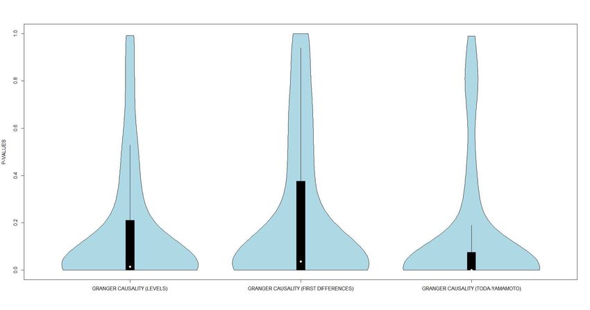
1     Introduction

The SARS-CoV-2 virus was initially detected in Wuhan (China) in December 2019 (Li et al. (2020a)),

and then rapidly spread to all Chinese provinces and the rest of the world in the subsequent months.

This chain of events led the World Health Organization (WHO, 2020) to declare a pandemic for the

Coronavirus disease (COVID-19) on the 11/03/2020. At the end of May 2020, confirmed coronavirus

cases worldwide surpassed 4 million and there were at least 300000 deaths in more than 180 countries

(ECDC, 2020).

    A large literature investigated how internet search data from search engines and data from traditional

surveillance systems can be used to compute real-time and short term forecasts of several diseases, see

Ginsberg et al. (2009), Broniatowski et al. (2013), Yang et al. (2015), and Santillana et al. (2015):

these approaches could predict the dynamics of disease epidemics several days or weeks in advance.

Besides, there is a small but quickly increasing literature that examines how internet search data can

be used to predict the COVID-19 pandemic, see for example Li et al. (2020b) and Ayyoubzadeh et al.

(2020). Moreover, to the best of our knowledge, neither formal Granger causality testing was computed

to determine whether Google search data is useful for forecasting COVID-19 cases, nor large scale out-

of-sample forecasting analysis was performed. The possibility to predict the dynamics of a dangerous

pandemic is of fundamental importance for policymakers and health officials to prevent its further spread

and to evaluate the success of their policy actions to contain the disease.

    In this study, we evaluated the ability of Google search data to forecast the number of new daily cases

and deaths of COVID-19 using data for 158 countries and a set of 18 forecasting models.

    The first contribution of this paper is an evaluation of the contribution of online search queries to the

modelling of the new daily cases of COVID- for 158 countries, using lag correlations between confirmed

cases and Google data, as well as different types of Granger causality tests. To our knowledge, this

analysis has not been done elsewhere. The second contribution is an out-of-sample forecasting exercise

with 18 competing models with a forecast horizon of 14 days ahead for all countries, with and without

Google data. The third contribution of the paper is a robustness check to measure the accuracy of the

models’ forecasts when forecasting the number of new daily deaths instead of cases.

    The rest of this paper is organized as follows. Section 2 briefly reviews the literature devoted to

forecasting infectious diseases with Google Trends and online data, while the methods proposed for

forecasting the new daily cases and deaths of COVID-19 are discussed in Section 3. The empirical results

are reported in Section 4, while a robustness check is discussed in Section 5. Section 6 briefly concludes.

                                                      2
2     Literature review

Several authors examined the predictive power of online data to forecast the temporal dynamics of differ-

ent diseases. They found that these data can offer significant improvements with respect to traditional

models: see, just to name a few, Ginsberg et al. (2009), Wilson et al. (2009), Seifter et al. (2010),

Valdivia and Monge-Corella (2010), Zhou and Feng (2011), Yin and Ho (2012), Ayers et al. (2013),

Yuan et al. (2013), Dugas et al. (2013), Majumder et al. (2016), Shin et al. (2016), Marques-Toledo et

al. (2017), Teng et al. (2017), Ho et al. (2018), Gianfredi et al. (2018), Santangelo et al. (2019), Li et

al. (2020b).

    Milinovich et al. (2014) provides one of the first and largest reviews of this literature and explains

the main reasons behind the predictive power of online data. The idea is quite simple: people suspecting

an illness tend to search online for information about the symptoms and, if possible, how they can self-

medicate. The last reason is particularly important in those countries where basic universal health care

and/or paid sick leave are not available.

    Traditional epidemiologic models to forecast infectious diseases may lack flexibility, be computation-

ally demanding, or require data that are not available in real-time, thus strongly reducing their practical

utility: see, for example, Longini et al. (1986), Hall et al. (2007), Birrell et al. (2011), Boyle et al.

(2011), and Dugas et al. (2013).

    Instead, internet-based surveillance systems are generally easy to compute and they are economically

affordable even for poor countries. Moreover, they can be used together with traditional surveillance

approaches. However, internet-based surveillance systems have also important limitations: they can

be strongly influenced by the mass media, which can push frightened people to search for additional

information online, thus misrepresenting the real situation on the ground. This is what happened during

the 2012-2013 influenza season, when Google Flu Trends (GFT) overestimated the prevalence of influenza

by more than fifty percent, see Lazer et al. (2014) for more details. Therefore, internet-based systems

should not be viewed as an alternative to traditional surveillance systems, but rather an extension.

Moreover, they can improve the ability to forecast the temporal dynamics of dangerous illnesses when

official statistics are not available or available with a delay, and when official statistics may not be fully

reliable.

    We remark that already in the middle of 2020 there is a very large literature devoted to forecasting

techniques for the COVID?19 disease. Shinde et al. (2020) provide a state-of-the-art survey of this

literature by reviewing 47 papers, including both published papers and pre-prints without peer-review.

They categorize these papers into 4 categories: (a) Big data; (b) Social media/other communication

media data; (c) Stochastic theory/mathematical models; (d) Data science/Machine learning techniques.

                                                      3
They examined each paper focusing on the specific countries used for the analysis, the various statistical,

analytical, mathematical and medical (symptomatic and asymptomatic) parameters taken into consid-

eration in the paper, and the main outcomes of the paper. Interestingly, despite several useful findings,

Shinde et al. (2020) highlight that there are still issues and challenges which need to be addressed.

The first and most important issue is the excessive reliance on China’s dataset for model testing and

forecasting, and the need to consider different datasets to verify “. . . whether the same mathematical or

prediction model is also suitable to predict the spread and reproduction number for all the countries across

the globe” (Shinde et al. (2020), p. 197). This was by far the most important driver behind the writing

of this paper, and which guided our research effort. Moreover, other challenges identified by Shinde et

al. (2020, p. 197) like longer incubation period, lack of proper data, over-fitting of the data, overly clean

data and model complexity influenced our choices in terms of model selection and data sources: these

issues will be discussed in more details in section 3 and 4.1, respectively.

    Gencoglu and Gruber (2020) were the first to try to discover and quantify causal relationships be-

tween the number of infections and deaths and online sentiment as measured by Twitter activity. This

is important because distinguishing epidemiological events that correlate with public attention from epi-

demiological events that cause public attention is fundamental when preparing public health policies.

However, Gencoglu and Gruber (2020) did not attempt to model temporal causal relationships: this

was one of the main reason why we decided to consider different types of Granger causality tests in our

analysis, as discussed below in section 3.1.

    Finally, we note that there is a strand of the literature that extends classical epidemiologic models

to study the interaction between economic decisions and epidemics, see Eichenbaum et al. (2020 a,b,c)

for more details. These works abstract from many important real-world complications to focus on the

basic economic forces at work during an epidemic, and to show that “there is an inevitable trade-off

between the severity of the short-run recession caused by the epidemic and the health consequences of that

epidemic” (Eichenbaum et al. (2020a), page 28). Given that these models are more intended for policy

making rather than forecasting, we did not consider them for this work.

3     Methodology

The goal of this paper is to verify whether Google Trends data is useful for forecasting new daily

cases/deaths of COVID-19. To this end, we will compute Granger causality tests and a large-scale

out-of-sample forecasting analysis. Before presenting the results of the empirical analysis, we briefly

review the theory of Granger causality testing and the forecasting models that we will use to predict the

daily cases and deaths of COVID-19.

                                                     4
3.1 Granger Causality
3.1.1 Brief review of the theory
Wiener (1956) was the first to propose the idea that, if the prediction of one time series can be improved
by using the information provided by a second time series, then the latter is said to have a causal influence
on the first. Granger (1969, 1980) formalized this idea in the case of linear regression models. In general,
if a variable (or a set of variables) X can improve forecasting another variable (or a set of variables) Y,
then we say that X Granger-causes Y. Otherwise, X fails to Granger-cause Y.
Let’s consider a general setting for a VAR(p) process with n variables,
Yt = α + Φ1 Yt−1 +Φ2 Yt−2 + · · · +Φp Yt−p + εt
with Yt , α, and εt n-dimensional vectors and Φi an n×n matrix of autoregressive parameters for lag i.
The VAR(p) process can be written more compactly as,
Y = BZ + U
where Y= (Y 1 , . . . , Y T ) is a (n × T ) matrix, B = (α, Φ1 , . . . , Φp ) is a (n×(1+np)) matrix, Z =
(Z 0 , . . . , ZT −1 ) is a ((1+np) × T ) matrix with Zt =[1 Y t . . . Y t−p+1 ]′ a (1+np) vector, and U =
(ε1 , . . . , εT ) is a (n × T ) matrix of error terms. If we want to test for Granger-causality, we need to test
a set of zero constraints on the coefficients: for example, the k -th element of Yt does not Granger-cause
the j -th element of Yt if the row j, column k element in Φi equals zero for i =1. . . p. More generally,
if we define β = vec(B) as a (n 2 p + n) vector with vec representing the column-stacking operator, the
null hypothesis of no Granger-causality can be expressed as
H0 : Cβ = 0 vs H1 : Cβ 6= 0,
where C is an (N ×(n 2 p + n)) matrix, 0 is an (N ×1) vector of zeroes, and N is the total number of
coefficients restricted to zero. It is possible to show that the Wald statistic defined by
′ h i−1
b b U )C b → d
χ2N
−1
Cβ C((ZZ) ⊗Σ Cβ (1)
b is the vector of estimated param-
has an asymptotic χ2 distribution with N degrees of freedom, where β
b U is the estimated covariance matrix of the residuals, see Lütkepohl (2005) –section 3.6.1–
eters, while Σ
for a proof.
53.1.2 Dealing with non-stationary data: the Toda–Yamamoto approach
It is well known that the use of non-stationary data can deliver spurious causality results, see Granger
and Newbold (1974), Phillips (1986), Park and Phillips (1989), Stock and Watson (1989), and Sims et al.
(1990). Moreover, Sims et al. (1990) showed that the asymptotic distribution theory cannot be applied
for testing causality even in the case when the variables are cointegrated.
Toda and Yamamoto (1995) introduced a Wald test statistic that asymptotically has a chi-square
distribution even if the processes may be integrated or cointegrated of arbitrary order. Their approach
requires, first, to determine the optimal VAR lag length p for the variables in levels using information
criteria. Secondly, a (p + d )th-order VAR is estimated, where d is the maximum order of integration
for the set of variables. Finally, Toda and Yamamoto (1995) showed that we can test linear or nonlinear
restrictions on the first p coefficient matrices using standard asymptotic theory, while the coefficient
matrices of the last d lagged vectors can be disregarded. Therefore, after a VAR(p+d ) model is estimated,
b = vec(α, Φ
the vector of the stacked estimated parameters can be modified as β b 1 , . . . ,Φ
b p , 0n×nd ),
where 0n×nd denotes a zero matrix with n rows and nd columns, and equation (1) can then be used.
Note that there are special cases when the extra lag(s) are not necessary to obtain the asymptotic
χ2 -distribution of the Wald test for Granger-causality, see Lütkepohl (2005) –section 7.6.3– for more
details.
3.2 Forecasting methods
We will perform an out-of-sample forecasting analysis for each country, to predict the number of daily
new cases and deaths using three classes of models: time series models, Google-augmented time series
models and epidemiologic models. A brief description of each model is reported below.
3.2.1 Time series models
Auto-Regressive Integrated Moving Average (ARIMA) models represent an important benchmark
in time series analysis and we refer the interested reader to Hamilton (1994) for a detailed discussion at the
textbook level. For sake of generality and interest (see section 4.1 below for more details)7, we considered
models with the variables in levels, log-levels, first differences and log-returns. The optimal number of
lags for the auto-regressive and moving average terms were chosen by minimizing the Akaike information
criteria (AIC). ARIMA models are important benchmarks in the famous forecasting competitions known
as Makridakis Competitions (or M-Competitions1 ), see Makridakis and Hibon (2000) and Makridakis et
al. (2020) for more details.
1 https://en.wikipedia.org/wiki/Makridakis Competitions
6Exponential smoothing methods have a long tradition in the statistical literature: recently, they
have witnessed a revival due to their inclusion in a general dynamic nonlinear framework, which allows
their implementation into state space form with several extensions, see Hyndman et al. (2002) and
Hyndman et al. (2008). This more general class of models is known as ETS (Error-Trend-Seasonal
or ExponenTial Smoothing ), and it includes standard exponential smoothing models, like the Holt
and Holt-Winters additive and multiplicative methods. The general structure of this framework is to
decompose a time series Y into three components: a trend (T ) which represents the long-term component
of Y, a seasonal pattern (S ), and an error term (E ). These components can enter the model specification
as additive terms (for example Y=T+S+E ), multiplicative (for example Y=T·S·E ) or both (for example,
Y=T·S+E ). Moreover, the trend component can be decomposed into a level term (l ) and a growth term
(b) which can be ”damped” by using an additional parameter 0< φ < 1 , so that five different trend
types are possible: 1) None: Th = l ; 2) Additive: Th = l + bh ; 3) Additive damped: Th = l + bφh ;
4) Multiplicative: Th = l · bh ; 5) Multiplicative damped: Th = l · bφh , where Th is the trend forecast h
Ph
periods out, while φh = s=1 φs . Therefore, we can have 30=5·3·2 possible ETS models, see Hyndman
et al. (2008) for more details.
Assuming a general state vector xt = [lt , bt , st , st−1 , . . . , st−m ] where lt , bt are the previous trends
components and st the seasonal terms, a state-space representation with a common error term of an
exponential smoothing model can be written as follows:
yt = h(xt−1 ) + k(xt−1 )εt
xt = f (xt−1 ) + g(xt−1 )εt
where h and k are continuous scalar functions, f and g are functions with continuous derivatives and
εt ∼N ID(0,σ 2 ). The equation for yt shows how the various state variable components (lt−1 , bt−1 , st−1 , . . .)
are combined to express yt as a function of a smoothed forecast ŷt =h(xt−1 ) with an error term εt , while
the equation for xt show how these state variable components are updated. The detailed equations for
all the 30 possible ETS models are reported in Hyndman et al. (2008) - Tables 2.2 and 2.3, p. 21-22.
ETS models are estimated by maximizing the likelihood function with multivariate Gaussian inno-
vations. Hyndman et al. (2008) showed that twice the negative logarithm of the likelihood function
conditional on the model parameters θ and the initial states x0 = (l0 , b0 , s0 , st−1 , . . . ) and without con-
stants, is given by: !
n
X n
X
∗ ε2
L (θ;x0 ) =nln +2 ln |k(xt−1 )|
t=1
k 2 (xt−1 ) t=1
The parameters θ and the initial states x0 are then estimated by minimizing L∗ (θ;x0 ). The model
7selection is then performed using information criteria. Like ARIMA models, the ETS model is also
an important benchmark in the famous M-competitions. Both ARIMA and ETS models provide good
forecasts in the short term, but the quality of these forecasts quickly decreases with an increasing forecast
horizon.
3.2.2 Google-augmented time series models
The easiest way to include Google search data in a time series model is probably by using an ARIMA
model with eXogenous variables (ARIMA-X), see Hyndman and Athanasopoulos (2018) for more
details. More specifically, we employed a simple ARIMA model augmented with the Google search data
for the topic ’pneumonia’ lagged by 14 days. This choice was based on two considerations: first, the WHO
(2020) officially states that “the time between exposure to COVID-19 and the moment when symptoms
start is commonly around five to six days but can range from 1 – 14 days”. Second, Li et al. (2020b)
showed that the daily new COVID-19 cases in China lag online search data for the topics ’coronavirus’
and ’pneumonia’ by 8-14 days, depending on the social platform used. We chose only the searches for
the topic ’pneumonia’ because they are less affected by news-only related searches. Even though such a
simple ARIMA-X model is definitely biased, this parsimonious model can nevertheless be of interest for
forecasting purposes. Moreover, the capacity of Google data to summarize a wealth of information should
not be underestimated, as shown by Fantazzini (2014) and Fantazzini and Toktamysova (2015). Similarly
to the previous ARIMA models, we considered four ARIMA-X models with the variables in levels, log-
levels, first differences and log-returns. We remind the reader that Google Trends data represents the
number of searches in Google for a topic or a keyword divided by the total amount of searches for the
same period and region, and standardized between 0 and 100. A detailed description of how this variable
is computed and some examples are reported in the Appendix A in the Supplementary Materials2 .
A more general framework is a trivariate VAR(p) model ,
p
X
Yt = ν + Φi Yt−i + ut , ut ∼ W N (0, Σu ) ,
i=1
where Yt is a (3 × 1)-vector containing the daily new cases of COVID-19 on day t, the daily Google
search data for the topics ’coronavirus’ and ’pneumonia’ filtered using the ’Health’ category to avoid
news-related searches, ν is an intercept vector, while Φi are the usual coefficient matrices with i =1,. . . ,p.
Similarly to ARIMA models, we considered four possible VAR(p) with the variables in levels, log-levels,
first differences and log-returns, while the optimal lags were again selected using the Akaike information
criteria. Given the small sample size at our disposal, higher-dimensional system were not considered
2 The supplementary materials can be found on the author’s website.
8because VAR(p) models suffer from the curse of dimensionality (the number of the parameters is equal
to k +pk 2 , where k is the number of time series). Similarly, we excluded cointegrated-VAR models due to
their computational problems with small samples and noisy Google data, see Fantazzini and Toktamysova
(2015) –section 4.4–, Fantazzini (2019) –section 7.6– and references therein for more details.
Unfortunately, even a simple trivariate VAR(p) can have a wealth of parameters: for example, if p=14,
129 parameters need to be estimated, which may be very difficult if not impossible to do, depending on
the sample size. It is for this reason, that the Hierarchical Vector Autoregression (HVAR) model
estimated with the Least Absolute Shrinkage and Selection Operator (LASSO) proposed by
Nicholson et al. (2017) and Nicholson et al. (2018) is an ideal approach in the case of a large number of
parameters and a small dataset. Let us consider again the previous VAR(p) process,
p
X
Yt = ν + Φi Yt−i + ut , ut ∼ W N (0, Σu ) ,
i=1
where Yt is a (3 × 1)-vector containing the daily new cases of COVID-19, and the daily Google data for
the topics ’coronavirus’ and ’pneumonia’. The HVAR approach proposed by Nicholson et al. (2018) adds
structured convex penalties to the least squares VAR problem to induce sparsity and a low maximum
lag order, so that the optimization problem is given by
T p 2
X X
min Yt − ν − Φp Yt−i + λ (PY (Φ)) ,
ν,Φ
t=1 i=1 F
where kAkF denotes the Frobenius norm of matrix A (that is, the elementwise 2-norm), λ ≥ 0 is a
penalty parameter, while PY (Φ) is the group penalty structure on the endogenous coefficient matrices.
We used the elementwise penalty function,
3 X
X p
3 X
PY (Φ) = kΦij,l k2
i=1 j=1 l=1
which is the most general structure, allowing every variable in every equation to have its own maximum
lag, so that there can be 32 = 9 possible lag orders. The penalty parameter λ was estimated by sequential
cross-validation, see Nicholson et al. (2018, 2019) for the full details. We considered the HVAR model
with the variables in levels, log-levels, first differences and log-returns. An example of sparsity pattern
with a trivariate H-VAR(5) model computed with the elementwise penalty function is reported in Figure 1.
The HVAR model is a special case of a multivariate penalized least squares optimization problem, which
can be solved using iterative nonsmooth convex optimization, and which has been recently implemented
in the R package BigVAR by Nicholson et al. (2019).
9Figure 1: Example of a trivariate HVAR(5) sparsity pattern, computed with the elementwise penalty
function. Active coefficients are shaded, whereas white cells denotes coefficients set to zero.
3.2.3 Epidemiologic models
The SIR (Susceptible, Infected, Recovered) compartmental epidemic model , was originally
proposed by Kermack and McKendrick (1927). Despite its relatively simple assumptions, it is still
nowadays one of the main benchmark models in epidemiology, see Brauer and Castillo-Chavez (2012)
–chapter 9– for a discussion at the textbook level.
The SIR model assumes that the population is divided into three compartments, where susceptible
is a group of people who can be infected, infectious represents the infected people who can transmit
the infection to susceptible people but can recover from it, while recovered represents the people who
got immunity and cannot be infected again. The SIR model describes the number of people in each
compartment using a set of ordinary differential equations:
dS βIS
= −
dt N
dI βIS
= − γI (2)
dt N
dR
= γI
dt
where β models how quickly the disease can be transmitted and it is given by the probability of contact
multiplied by the probability of disease transmission, while γ models how quickly people recover from
the disease. Note that N = S (t) + I(t) + R(t) represents the total population and it is a constant. The
ratio R0 = β/γ is known as the basic reproduction number and it represents the average number of new
infected people from a single infected person. The interpretation of this number is easier if we consider
that 1/γ represents the average time needed to recover from the disease, while 1/β is the average time
between contacts.
The SIRD (Susceptible, Infectious, Recovered, Deceased ) model adds a fourth compartment
10to model the dynamics of deceased people:
dS βIS
= −
dt N
dI βIS
= − γI − µI (3)
dt N
dR
= γI
dt
dD
= µI
dt
where µ is the mortality rate. Anastassopoulou et al. (2020) were the first to use the SIRD model
with COVID-19 data. Even though several variants of the SIR model have been proposed, they require
additional information that is not publicly available or available with great delay. Moreover, the level of
numerical complexity is much higher and this may strongly penalize the efficiency of the model estimates:
this will be evident when we will compare the SIR and the SIRD models in section 5. I refer the interested
reader to Soetaert et al. (2010a,b) and Brauer and Castillo-Chavez (2012) for more details about the
estimation of systems of ordinary differential equations.
4 Empirical analysis
4.1 Data
The daily numbers of COVID-19 confirmed cases for over 200 countries were downloaded from the website
of the European Centre for Disease Prevention and Control (ECDC), which is an agency of the European
Union. To the author’s knowledge, this is probably the best COVID-19 dataset currently available. The
detailed procedure explaining how the data are collected is reported below for ease of reference:
“Since the beginning of the coronavirus pandemic, ECDC’s Epidemic Intelligence team has
been collecting on daily basis the number of COVID-19 cases and deaths, based on reports from
health authorities worldwide. To insure the accuracy and reliability of the data, this process is
being constantly refined. This helps to monitor and interpret the dynamics of the COVID-19
pandemic not only in the European Union (EU), the European Economic Area (EEA), but
also worldwide. Every day between 6.00 and 10.00 CET, a team of epidemiologists screens
up to 500 relevant sources to collect the latest figures. The data screening is followed by
ECDC’s standard epidemic intelligence process for which every single data entry is validated
and documented in an ECDC database. An extract of this database, complete with up-to-date
figures and data visualisations, is then shared on the ECDC website, ensuring a maximum
level of transparency”.
11https://data.europa.eu/euodp/en/data/dataset/covid-19-coronavirus-data
Additional comments about this dataset and other COVID-19 datasets can be found in Alamo et
al. (2020). We want to remark that only countries that had at least 100 confirmed cases at the time of
writing this paper were considered (that is, in May 2020).
Following Li et al. (2020b), we also downloaded the daily data related to the two specific search
terms ’coronavirus’ and ’pneumonia’ from Google Trends, using the time range 01/01/2020 - 13/05/20.
However, our Google dataset differs from Li et al. (2020b) in two aspects. First, we downloaded the data
relative to the topics in the place of the simple keywords: search data for topics are cleaned automatically
by Google of all searches that are not related to the specific chosen topic. Second, only topics data from
the ’Health’ category were considered, to avoid all news-related searches. These two filters were used
to reduce the noise in the data and improve their predictive ability. Note that the use of Google topics
solves automatically the problem of translating the keywords into local languages.
We remark that the issue of weekly seasonality, which is present in mild form both in daily COVID
data and in Google searches, was not dealt directly because the estimation of several models would have
become very difficult (if not impossible) if additional parameters were added to deal with seasonality.
However, we tried to deal with it at least partially in two ways: first, we considered the ETS model that
can model seasonality by construction. Had seasonality been an important factor, ETS models would
have out-performed the competitors, but this was not the case. Secondly, Google search data showed a
very mild seasonality (people searched more on the weekends than in working days), so that regressing the
number of daily cases/deaths against Google data was a simple and indirect way to deal with seasonality.
More complex and sophisticated approaches to deal with seasonality like those employed by Franses and
Paap (2004) would require much larger datasets that are currently not available. This is why we leave
this issue as an avenue for further research.
We want to emphasize that at the beginning of the pandemic the reproduction number was probably
above unity for many (if not all) countries, so that it is very likely that the processes generating the
COVID daily data series were explosive, that is with the unit root greater than one. In such a case, the
data are not integrable of any order (similarly to financial bubble processes), and the assumptions for
the unit root tests are not satisfied, so that the critical values of the tests may not be valid. However, the
effects on the test result strongly depend on the specific test used and the chosen alternative hypothesis
(either the stationary alternative or the explosive alternative), see Haldrup and Lildholdt (2002) for
details. Given this issue, we decided to take a neutral stance, and the subsequent empirical analysis
considered models for data in levels, log-levels, first-differences, and log-returns. In this regard, we
emphasize that a large part of the epidemiologic literature does not deal with non-stationarity at all, see
12Cazelles et al. (2018) and references therein for more details3 .
Following Li et al. (2020b), the first step of the empirical analysis was the computation of the lag
correlations between the daily COVID-19 cases for each country and Google search data for the topics
’coronavirus’ and ’pneumonia’ up to a 30-day horizon. The 30-day horizon was chosen based on the
limited size of our dataset and on past literature, see Lin et al. (2020) and references therein. For the
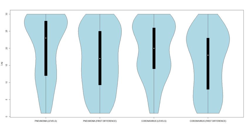
sake of space and interest, we report in Figure 2 the violin plots (that is, kernel densities + box plot) of
the lags showing the highest correlation between the daily COVID-19 cases and Google searches across
all countries, for both variables in levels and first-differences. Instead, the highest lagged correlations
together with their corresponding lags for each country are reported in the Supplementary Table S1 and
S2, for the case of variables in levels and in first differences, respectively4 .
Figure 2: Violin plots of the lags with the highest correlations between new COVID-19 cases and Google
searches for the topics ‘coronavirus’ and ‘pneumonia’ across 158 countries, January–May 2020.
Figure 2 shows that the median lag with the highest correlation across all countries is 23 days
(levels) / 17 days (first differences) for the ‘pneumonia’ topic, while it is 20 days (levels) / 18 days (first
differences) for the ‘coronavirus’ topic. In general, these results are fairly stable across data in levels and
first differences and quite close to those reported by Li et al. (2020b), even though somewhat higher
3 Testing for Granger causality using the Toda–Yamamoto (1995) approach should not particularly suffer from processes
that are mildly explosive and have this feature only at the beginning of the pandemic. This follows from Haldrup and
Lildholdt (2002), who showed that I(2) processes have properties that mimic those of explosive processes in finite samples,
and from the fact that the Toda–Yamamoto approach is valid with processes which may be integrated or cointegrated of
arbitrary order. Moreover, this approach has been found to be valid with a larger set of processes, as shown by the large
simulation studies performed by Hacker and Hatemi (2006).
4 The supplementary materials can be found on the author’s website.
13than the latter. In this regard, we remark again that the WHO (2020) states that “the time between
exposure to COVID-19 and the moment when symptoms start is commonly around five to six days but can
range from 1 – 14 days”. Moreover, the fact that infected people may wait some time before contacting
a doctor (fear of job loss, attempt to self-medicate, etc.), together with the objective difficulty to get
tested in several countries, can explain why the lags with the highest correlation are generally higher
than those reported for China by Li et al. (2020b).
4.2 Granger Causality
Even though lag-correlations are a useful tool to gain a general idea about potential predictability, it is
better to compute a Granger-causality (GC) test to formally test whether one (or more) time series can
be useful in forecasting another time series. The violin plots of the p-values for the null hypothesis that
Google searches for the topics ’coronavirus’ and ’pneumonia’ do not Granger-cause the daily new COVID-
19 cases, using vector auto-regressive models with optimal lags selected with the Akaike information
criteria (for both the variables in levels and in first differences), are reported in Figure 3. The same
figure also reports the p-values for the null hypothesis of no Granger-causality using the approach by
Toda-Yamamoto, which is valid even if the processes may be integrated or cointegrated of arbitrary
order.
Figure 3: Violin plots of the p-values for the null hypothesis that the Google searches for the topics
’coronavirus’ and ’pneumonia’ do not Granger-cause the daily new COVID-19 cases across 158 countries,
January–May 2020.
14The detailed p-values for the null hypothesis that the Google searches do not Granger-cause the
daily new COVID-19 cases across 158 countries are reported in the Supplementary Table S3: the null
hypothesis was rejected at the 5% probability level for 87 out of 158 countries using variables in levels,
for 80 countries using variables in first differences, and for 106 countries using the approach by Toda
and Yamamoto. Therefore, there is strong evidence that lagged Google search data do explain the
variation in the daily new COVID-19 cases for the vast majority of countries worldwide. It is interesting
to note that when we move to an approach like the Toda-Yamamoto methodology able to deal with
non-stationarity (and potentially explosive processes, given that I(2) processes mimic explosive processes
in finite samples), the evidence in favor of Google data further increases.
4.3 Out-of-sample forecasting
The last step to evaluate the ability of Google search data to predict the COVID-19 outbreak was to
perform an out-of-sample forecasting analysis for each country, to forecast the number of daily new cases
using several competing models with and without Google data. Three classes of models were considered
for a total of 18 models:
1. Time series models with the daily number of new COVID-19 cases as the dependent variable:
(a) ARIMA models with the variables in levels, log-levels, first differences and log-returns. Total:
4 models.
(b) Error-Trend-Seasonal (ETS) model. Total: 1 model.
2. Google-augmented time series models:
(a) ARIMA-X with lagged Google data for the topic ’pneumonia’ as an exogenous repressor, with
the variables in levels, log-levels, first differences and log-returns. Total: 4 models.
(b) VAR models with the variables in levels, log-levels, first differences and log-returns. The
endogenous regressors are the daily number of new COVID-19 cases and the Google search
data for the topics ’coronavirus’ and ’pneumonia’. Total: 4 models.
(c) The Hierarchical Vector Autoregression (HVAR) model estimated with the Least Absolute
Shrinkage and Selection Operator (LASSO), with the variables in levels, log-levels, first dif-
ferences and log-returns. Total: 4 models.
3. The SIR compartmental epidemic model. Total: 1 model.
15Additional models could surely be added, but this selection already gave important indications
whether Google search data are useful for forecasting the daily cases of COVID-19. Given the pre-
vious evidence with lag correlations and Granger-causality tests, a forecasting horizon of 14 days was
considered. Note that precise forecasts over a 2-week horizon can be extremely important for policy
makers and health officers.
The data in January-March 2020 were used as the first training sample for the models’ estimation,
while April-May 2020 was left for out-of-sample forecasting using an expanding estimation window. A
summary of the models’ performances across the 158 countries according to the mean squared error
(MSE) and the mean absolute error (MAE) is reported in Table 1, respectively, while the top 3 models
for each country are reported in the Supplementary Table S4 and Supplementary Table S5, respectively.
Number of times the model was:
MSE MAE
Models 1st best 2nd best 3rd best 1st best 2nd best 3rd best
Time series models ARIMA 7 9 21 5 17 16
ARIMA.LOG 16 15 7 20 17 18
ARIMA.DIFF 11 21 22 9 16 16
ARIMA.DIFFLOG 2 4 3 0 3 5
ETS 6 6 12 7 14 11
ARIMAX 9 13 17 7 11 17
ARIMAX.LOG 12 14 10 12 19 13
ARIMAX.DIFF 15 24 16 18 15 12
ARIMAX.DIFFLOG 13 3 7 8 3 7
VAR 0 0 0 0 0 0
Google- augmented VAR.LOG 1 0 1 1 0 1
time series models VAR.DIFF 0 0 0 0 0 0
VAR.DLOG 0 2 4 0 3 4
HVAR 15 5 6 11 5 7
HVAR.LOG 10 12 6 19 8 9
HVAR.DIFF 7 11 8 8 5 11
HVAR.DLOG 4 5 8 5 8 8
Compartmental epi- SIR 30 14 10 28 14 3
demic model
Table 1: Summary of the models’ performances across the 158 countries (according to the MSE and the
MAE) for the out-of-sample period in April-May 2020.
Google-augmented time series models were the best models for 86/89 countries out of 158 according to
the MSE/MAE (mainly ARIMA-X models and HVAR models). The SIR model confirmed its good name
by being the top model for almost 20% of the countries examined. There is no major differences between
models with the variables in levels and in first-differences, whereas models in log-levels seem to show
slightly better performances across different models’ specifications. VAR models performed very poorly
and in several occasions did not reach numerical convergence, due to the large number of parameters
involved with small sample sizes.
The previous loss functions were then used with the Model Confidence Set (MCS) by Hansen et al.
16(2011) to select the best forecasting models at a specified confidence level. Once the loss differential
between models i and j at time t are computed (that is di,j,t = Li,t −Lj,t ), the MCS approach tests
the hypothesis of equal predictive ability, H0,M : E(di,j,t ) = 0, for all i,j ∈ M, where M is the set
of forecasting models. First, the following t-statistics are computed, ti· =di· /d
v ar di· for i ∈ M, where
P
di· = m−1 j∈M dij is the simple loss of the i -th model relative to the average losses across models
PT
in the set M, dij = T −1 t=1 dij,t measures the sample loss differential between model i and j, and
vd
ar di· is an estimate of var di· . Secondly, the following test statistic is computed to test for the null
hypothesis: Tmax = maxi∈M (ti· ) . This statistic has a non-standard distribution, so the distribution
under the null hypothesis is computed using bootstrap methods with 2000 replications. If the null
hypothesis is rejected, one model is eliminated from the analysis and the testing procedure starts again.
The number of times each model was included into the MCS across the 158 countries, according to
the MSE and the MAE, is reported in Table 2.
Loss: MSE Loss: MAE
ARIMA 145 ARIMA 127
ARIMA.LOG 147 ARIMA.LOG 131
ARIMA.DIFF 145 ARIMA.DIFF 133
ARIMAX.DIFFLOG 130 ARIMAX.DIFFLOG 116
ETS 142 ETS 122
ARIMAX 144 ARIMAX 125
ARIMAX.LOG 146 ARIMAX.LOG 130
ARIMAX.DIFF 141 ARIMAX.DIFF 129
ARIMA.DIFFLOG 133 ARIMA.DIFFLOG 115
VAR 96 VAR 76
VAR.LOG 74 VAR.LOG 59
VAR.DIFF 99 VAR.DIFF 75
VAR.DLOG 102 VAR.DLOG 90
HVAR 138 HVAR 115
HVAR.LOG 138 HVAR.LOG 127
HVAR.DIFF 138 HVAR.DIFF 121
HVAR.DLOG 134 HVAR.DLOG 116
SIR 138 SIR 116
Table 2: Number of times each model was included into the MCS across the 158 countries.
With the exception of VAR models, almost all models were included in the MCS, thus showing that
there was not enough information in the data to partition good and bad models: this outcome was
expected given the small sample used in this forecasting exercise.
175 Robustness check: modelling and forecasting the number of
COVID-19 deaths
A common critique to the analysis of COVID-19 cases is that the number of cases could depend on the
amount of testes, so that a country could have few official cases due to low testing. Therefore, modelling
and forecasting the number of COVID-19 deaths could be a better metric to evaluate the forecasting
ability of Google search data. We repeated the previous analysis with the daily deaths for COVID-19,
considering only those countries with at least 100 deaths (for a total of 64 countries). The violin plots of
the lags with the highest correlations between new daily COVID-19 deaths and Google searches for the
topics ‘coronavirus’ and ‘pneumonia’ is reported in Figure 4. The violin plots of the p-values for the null
hypothesis that the Google searches for the topics ’coronavirus’ and ’pneumonia’ do not Granger-cause
the daily COVID-19 deaths across 158 countries is reported in Figure 5.
Figure 4: Violin plots of the lags with the highest correlations between daily COVID-19 deaths and
Google searches for the topics ‘coronavirus’ and ‘pneumonia’ across 158 countries, January–May 2020.
Figure 4 shows that the median lag with the highest correlation across all countries is 28 days (levels) /
19 days (first differences) for the ‘pneumonia’ topic, while it is 26 days (levels) / 18 days (first differences)
for the ‘coronavirus’ topic: the highest correlations in levels take place approximately 1 week later that
those for the confirmed cases, which makes sense from an epidemiologic point of view.
The null hypothesis that the Google searches do not Granger-cause the daily new COVID-19 deaths
across 64 countries was rejected at the 5% probability level for 40 countries using variables in levels, for
18Figure 5: Violin plots of the p-values for the null hypothesis that the Google searches for the topics
’coronavirus’ and ’pneumonia’ do not Granger-cause the daily COVID-19 deaths across 158 countries,
January–May 2020.
30 countries using variables in first differences, and for 42 countries using the approach by Toda and
Yamamoto. Therefore, there is strong evidence that lagged Google search data do explain the variation
in the daily new COVID-19 deaths for most of the countries examined.
The out-of-sample forecasting analysis involved again the previous 17 time series models, but they
used the daily number of new COVID-19 deaths as the dependent variable, instead. As for epidemiologic
models, we considered two variants:
a) the SIR model described by the system of equations 2 where the number of infected is substituted
with the number of deaths, thus implying that the mortality rate for those infected is 100%. This is
clearly a biased (and unrealistic) model, but it has a benefit to be numerically more efficient than more
complex epidemic models. Moreover, it can be interpreted as a shrinkage estimator, see Lehmann and
Casella (1998);
b) the SIRD model described by the system of equations 3, which is a benchmark model in epidemi-
ology when both people infected and deaths have to be modelled.
A summary of the models’ performances across the 64 countries according to the mean squared error
(MSE) and the mean absolute error (MAE) is reported in Table 3.
Google-augmented time series models were the best models for 38/39 countries out of 64 according
to the MSE/MAE (again ARIMA-X models and HVAR models). There is no major differences between
models with the variables in levels and in first-differences, but ARIMA-X models in first differences seem
19MSE MAE
Models 1st best 2nd best 3rd best 1st best 2nd best 3rd best
ARIMA 5 11 6 2 9 8
ARIMA.LOG 1 2 3 2 8 6
Time series models ARIMA.DIFF 5 7 7 7 6 8
ARIMA.DIFFLOG 2 7 3 1 5 4
ETS 2 0 0 1 2 2
ARIMAX 3 5 8 8 3 3
ARIMAX.LOG 1 1 4 2 5 5
ARIMAX.DIFF 17 7 5 13 10 3
ARIMAX.DIFFLOG 4 4 2 5 1 1
Google- augmented VAR 0 0 0 0 0 0
time series models VAR.LOG 0 0 0 0 0 1
VAR.DIFF 0 0 0 0 0 0
VAR.DLOG 1 0 1 0 1 1
HVAR 5 2 4 6 4 2
HVAR.LOG 1 2 0 1 1 1
HVAR.DIFF 4 4 6 1 5 7
HVAR.DLOG 2 4 6 3 2 5
Compartmental SIR 8 7 9 11 2 7
epidemic model SIRD 3 1 0 1 0 0
Table 3: Summary of the models’ performances when forecasting the daily deaths for COVID-19 across
the 64 countries (according to the MSE and the MAE) for the out-of-sample period in April-May 2020.
to show better performances than competing models. VAR models performed again very poorly. The SIR
and SIRD model were the top models for approximately 18% of the countries examined: interestingly, the
SIR model performed better than the SIRD model, thus confirming again that in some cases efficiency
is more important than unbiasedness.
The number of times each model was included into the MCS across the 64 countries -according to
the MSE and the MAE- is reported in Table 4:
Loss: MSE Loss: MAE
ARIMA 61 ARIMA 58
ARIMA.LOG 58 ARIMA.LOG 52
ARIMA.DIFF 61 ARIMA.DIFF 57
ARIMA.DIFFLOG 53 ARIMA.DIFFLOG 54
ETS 54 ETS 48
ARIMAX 59 ARIMAX 54
ARIMAX.LOG 57 ARIMAX.LOG 51
ARIMAX.DIFF 60 ARIMAX.DIFF 59
ARIMAX.DIFFLOG 47 ARIMAX.DIFFLOG 44
VAR 21 VAR 19
VAR.LOG 16 VAR.LOG 20
VAR.DIFF 25 VAR.DIFF 22
VAR.DLOG 22 VAR.DLOG 26
HVAR 54 HVAR 50
HVAR.LOG 53 HVAR.LOG 42
HVAR.DIFF 58 HVAR.DIFF 56
HVAR.DLOG 58 HVAR.DLOG 53
SIR 59 SIR 52
SIRD 48 SIRD 35
Table 4: Number of times each model was included into the MCS across the 64 countries.
Similarly to the baseline case, almost all models were included in the MCS (with the exception of
20VAR models, and the SIRD model to a lower degree), thus showing again that there was not enough
information in the data to separate good and bad models.
6 Conclusions
Google Trends data for the topics ’coronavirus’ and ’pneumonia’ filtered using the ’Health’ category
proved to be strongly predictive for the number of new daily cases and deaths of COVID-19 for a large
set of countries. Google data can complement epidemiological models during difficult times like the
ongoing COVID-19 pandemic, when official statistics maybe not fully reliable and/or published with a
delay. Policymakers and health officials can use web searches to verify how the pandemic is developing,
and/or to check the effect of their policy actions to contain the disease and to modify them if these policies
prove to be unsatisfactory. This is particularly important now that several countries have decided to
reopen their economies, so that real-time tracking with online-data is one of the instruments that can be
used to keep the situation under control.
Even though some models performed better than others did, these forecasting differences were not
statistically significant due to the small samples used. An avenue of future research would be to con-
sider larger samples and forecast combination methods, following the ideas discussed by Clemen (1989),
Timmermann (2006), Hsiao and Wan (2014), and Hyndman and Athanasopoulos (2018).
21References
Alamo T., Reina D.G., Mammarella M., Abella A. (2020). Covid-19: Open-Data Resources for Monitoring, Modeling, and
Forecasting the Epidemic. Electronics, 9(5), 827.
Anastassopoulou C., Russo L., Tsakris A., Siettos C. (2020). Data-based analysis, modelling and forecasting of the
COVID-19 outbreak. PloS one, 15(3), e0230405.
Ayers J.W., Althouse B.M., Allem J.P., Rosenquist J.N., Ford D.E. (2013). Seasonality in seeking mental health
information on Google. American Journal of Preventive Medicine, 44(5), 520-525.
Ayyoubzadeh S.M., Ayyoubzadeh S.M., Zahedi H., Ahmadi M., Kalhori, S.R.N. (2020). Predicting COVID-19 incidence
through analysis of google trends data in iran: data mining and deep learning pilot study. JMIR Public Health and
Surveillance, 6(2), e18828.
Birrell P.J., Ketsetzis G., Gay N.J., Cooper B.S., Presanis A.M., Harris R.J, Charlett A., Zhang X.S., White P.,
Pebody R., De Angelis D. (2011). Bayesian modeling to unmask and predict influenza A/H1N1pdm dynamics in London.
Proceedings of the National Academy of Sciences, 108(45), 18238-18243.
Boyle J.R., Sparks R.S., Keijzers G.B., Crilly J. L., Lind J. F., Ryan L.M. (2011). Prediction and surveillance of
influenza epidemics. Medical journal of Australia, 194, S28-S33.
Brauer F., Castillo-Chavez C., Castillo-Chavez C. (2012). Mathematical models in population biology and epidemiology.
New York: Springer.
Broniatowski D.A., Paul M.J., Dredze M. (2013). National and local influenza surveillance through Twitter: an analysis
of the 2012-2013 influenza epidemic. PloS one, 8(12).
Cazelles B., Champagne C., Dureau J. (2018). Accounting for non-stationarity in epidemiology by embedding time-
varying parameters in stochastic models. PLoS computational biology, 14(8), e1006211.
Clemen R.T. (1989). Combining forecasts: A review and annotated bibliography. International journal of forecasting,
5(4), 559-583.
Costantini M., Lupi C. (2013). A Simple Panel?CADF Test for Unit Roots. Oxford Bulletin of Economics and
Statistics, 75(2), 276-296.
D’Amuri F., Marcucci J. (2017). The predictive power of Google searches in forecasting US unemployment. Interna-
tional Journal of Forecasting, 33(4), 801-816.
Dugas A.F., Jalalpour M., Gel Y., Levin S., Torcaso F., Igusa T., Rothman R.E. (2013). Influenza forecasting with
Google flu trends. PloS one, 8(2), e56176.
Eichenbaum M.S., Rebelo S., Trabandt M. (2020a). The Macroeconomics of Epidemics. National Bureau of Economic
Research, No. w26882.
Eichenbaum M.S., Rebelo S., Trabandt M. (2020b). The Macroeconomics of Testing and Quarantining. National
Bureau of Economic Research, No. w27104.
Eichenbaum M.S., Rebelo S., Trabandt M. (2020c). Epidemics in the Neoclassical and New Keynesian Models. National
Bureau of Economic Research, No. w27430.
European Centre for Disease Prevention and Control (ECDC, 2020). Download today’s data on the geographic distri-
bution of COVID-19 cases worldwide. Available from:
https://www.ecdc.europa.eu/en/publications-data/download-todays-data-geographic-distribution-covid-19-cases-worldwide.
Accessed on May 1 2020.
Fantazzini D. (2014). Nowcasting and forecasting the monthly food stamps data in the US using online search data.
PloS one, 9(11), e111894.
Fantazzini, D. (2019). Quantitative finance with R and cryptocurrencies. Amazon KDP, ISBN-13, 978-1090685315.
Fantazzini D., Toktamysova Z. (2015). Forecasting German car sales using Google data and multivariate models.
International Journal of Production Economics, 170, 97-135.
Franses P.H., Paap R. (2004). Periodic time series models. OUP Oxford.
Gianfredi V., Bragazzi N.L., Mahamid M., Bisharat B., Mahroum N., Amital H., Adawi M. (2018). Monitoring public
interest toward pertussis outbreaks: an extensive Google Trends–based analysis. Public Health, 165, 9-15.
Ginsberg J., Mohebbi M.H., Patel R.S., Brammer L., Smolinski M.S., Brilliant L. (2009). Detecting influenza epidemics
using search engine query data. Nature, 457(7232), 1012-1014.
Granger C.W. (1969). Investigating causal relations by econometric models and cross-spectral methods. Econometrica,
424-438.
Granger C.W. (1980). Testing for causality: a personal viewpoint. Journal of Economic Dynamics and control, 2,
329-352.
Granger C.W., Newbold P. (1974). Spurious regressions in econometrics, Journal of Econometrics, 2, 111– 120.
22Hacker R.S., Hatemi J.A. (2006). Tests for causality between integrated variables using asymptotic and bootstrap
distributions: theory and application. Applied Economics, 38(13), 1489-1500.
Haldrup N., Lildholdt P. (2002). On the robustness of unit root tests in the presence of double unit roots. Journal of
Time Series Analysis, 23(2), 155-171.
Hall I.M., Gani R., Hughes H.E., Leach S. (2007). Real-time epidemic forecasting for pandemic influenza. Epidemiology
and Infection, 135(3), 372-385.
Hansen P.R., Lunde A., Nason J.M. (2011). The model confidence set. Econometrica, 79(2), 453–497.
Ho H.T., Carvajal T.M., Bautista J.R., Capistrano J.D.R., Viacrusis K.M., Hernandez L.F.T., Watanabe K. (2018).
Using Google Trends to examine the spatio-temporal incidence and behavioral patterns of dengue disease: A case study in
Metropolitan Manila, Philippines. Tropical medicine and infectious disease, 3(4), 118.
Hsiao C., Wan S.K. (2014). Is there an optimal forecast combination? Journal of Econometrics, 178, 294-309.
Hyndman R.J., Koehler A.B., Snyder R.D., Grose,S. (2002). A state space framework for automatic forecasting using
exponential smoothing methods. International Journal of forecasting, 18(3), 439-454.
Hyndman R., Koehler A.B., Ord J.K., Snyder R.D. (2008). Forecasting with exponential smoothing: the state space
approach. Springer Science and Business Media.
Hyndman R.J., Athanasopoulos G. (2018). Forecasting: principles and practice. OTexts.
Im K.S., Pesaran M.H., Shin Y. (2003). Testing for unit roots in heterogeneous panels. Journal of econometrics,
115(1), 53-74.
Kermack W.O., McKendrick A. G. (1927). A contribution to the mathematical theory of epidemics. Proceedings of
the royal society of london. Series A, 115(772), 700-721.
Lazer D., Kennedy R., King G., Vespignani A. (2014). The parable of Google Flu: traps in big data analysis. Science,
343(6176), 1203-1205.
Lehmann E.L., Casella G. (1998). Theory of point estimation. Springer Science and Business Media.
Levin A., Lin C. F., Chu C.S.J. (2002). Unit root tests in panel data: asymptotic and finite-sample properties. Journal
of econometrics, 108(1), 1-24.
Li Q., Guan X., Wu P., Wang X., Zhou L., Tong Y., Ren R, Leung K.S., Lau E.H., Wong J.Y., Xing X. (2020a). Early
transmission dynamics in Wuhan, China, of novel coronavirus–infected pneumonia. New England Journal of Medicine,
382(13), 1199-1207.
Li C., Chen L.J., Chen X., Zhang M., Pang C.P., Chen H. (2020b). Retrospective analysis of the possibility of predicting
the COVID-19 outbreak from Internet searches and social media data, China, 2020. Eurosurveillance, 25(10), 2000199.
Longini I.M., Fine P.E., Thacker S.B. (1986). Predicting the Global Spread of new infectious agents. American Journal
of Epidemiology, 123(3): 383-39.
Lütkepohl, H. (2005). New introduction to multiple time series analysis. Springer Science and Business Media.
Maddala G.S., Wu S. (1999). A comparative study of unit root tests with panel data and a new simple test. Oxford
Bulletin of Economics and statistics, 61(S1), 631-652.
Makridakis S., Hibon M. (2000). The M3-Competition: results, conclusions and implications. International journal of
forecasting, 16(4), 451-476.
Makridakis S., Spiliotis E., Assimakopoulos V. (2020). The M4 Competition: 100,000 time series and 61 forecasting
methods. International Journal of Forecasting, 36(4), 54-74.
Majumder M.S., Santillana M., Mekaru S.R., McGinnis D.P., Khan K., Brownstein J.S. (2016). Utilizing nontraditional
data sources for near real-time estimation of transmission dynamics during the 2015-2016 Colombian Zika virus disease
outbreak. JMIR public health and surveillance, 2(1), e30.
Milinovich G.J., Williams G.M., Clements A.C., Hu W. (2014). Internet-based surveillance systems for monitoring
emerging infectious diseases. The Lancet infectious diseases, 14(2), 160-168.
Marques-Toledo C., Degener C.M., Vinhal L., Coelho G., Meira W., Codeço C.T., Teixeira M.M. (2017). Dengue
prediction by the web: Tweets are a useful tool for estimating and forecasting Dengue at country and city level. PLoS
neglected tropical diseases, 11(7), e0005729.
Nicholson W.B., Matteson D.S., Bien J. (2017). VARX-L: Structured regularization for large vector autoregressions
with exogenous variables. International Journal of Forecasting, 33(3), 627-51.
Nicholson W. B., Wilms I., Bien J., Matteson D. S. (2018). High dimensional forecasting via interpretable vector
autoregression. arXiv preprint, arXiv:1412.5250
Nicholson, w., Matteson, D., and Bien, J. (2019). BigVAR: Dimension Reduction Methods for Multivariate Time
Series. R package version 1.0.6.
23You can also read