Seasonal glacier and snow loading in Svalbard recovered from geodetic observations
←
→
Page content transcription
If your browser does not render page correctly, please read the page content below
Geophys. J. Int. (2022) 229, 408–425                                                                                 https://doi.org/10.1093/gji/ggab482
Advance Access publication 2021 November 27
GJI Gravity, Geodesy and Tides

Seasonal glacier and snow loading in Svalbard recovered from
geodetic observations

H.P. Kierulf,1,2 W.J.J. van Pelt,3 L. Petrov,4 M. Dähnn,1 A.-S. Kirkvik1 and O. Omang1
1 GeodeticInstitute, Norwegian Mapping Authority, 3507 Hønefoss, Norway. E-mail: halfdan.kierulf@kartverket.no
2 Department of Geosciences, University of Oslo, 0371 Oslo, Norway
3 Department of Earth Sciences, Uppsala University, 752 36 Uppsala, Sweden
4 NASA Goddard Space Flight Center, Greenbelt, MD 20771, USA

                                                                                                                                                             Downloaded from https://academic.oup.com/gji/article/229/1/408/6445027 by guest on 27 February 2022
Accepted 2021 November 25. Received 2021 May 10; in original form 2021 November 23

                                       SUMMARY
                                       We processed time-series from seven Global Navigation Satellite System (GNSS) stations and
                                       one Very Long Baseline Interferometry (VLBI) station in Svalbard. The goal was to capture
                                       the seasonal vertical displacements caused by elastic response of variable mass load due to
                                       ice and snow accumulation. We found that estimates of the annual signal in different GNSS
                                       solutions disagree by more than 3 mm which makes geophysical interpretation of raw GNSS
                                       time-series problematic. To overcome this problem, we have used an enhanced Common Mode
                                       (CM) filtering technique. The time-series are differentiated by the time-series from remote
                                       station BJOS with known mass loading signals removed a priori. Using this technique, we
                                       have achieved a substantial reduction of the differences between the GNSS solutions. We have
                                       computed mass loading time-series from a regional Climatic Mass Balance (CMB) and snow
                                       model that provides the amount of water equivalent at a 1 km resolution with a time step of 7 d.
                                       We found that the entire vertical loading signal is present in data of two totally independent
                                       techniques at a statistically significant level of 95 per cent. This allowed us to conclude that the
                                       remaining errors in vertical signal derived from the CMB model are less than 0.2 mm at that
                                       significance level. Refining the land water storage loading model with a CMB model resulted
                                       in a reduction of the annual amplitude from 2.1 to 1.1 mm in the CM filtered time-series, while
                                       it had only a marginal impact on raw time-series. This provides a strong evidence that CM
                                       filtering is essential for revealing local periodic signals when a millimetre level of accuracy is
                                       required.
                                       Key words: Glaciology; Global change from geodesy; Loading of the Earth; Reference
                                       systems; Satellite geodesy; Arctic region.

                                                                               1990s with Global Navigation Satellite System (GNSS) antennas,
1 I N T RO D U C T I O N
                                                                               Very Long Baseline Interferometry (VLBI) telescope, Super Con-
The Arctic archipelago Svalbard is exposed to climate change phe-              ducting Gravity (SCG), absolute gravity points and control networks
nomena, the temperature is rising, the permafrost is melting, the              (Kierulf et al. 2009a).
sea level is rising and the glaciers are retreating (Hanssen-Bauer                Due to Svalbard’s remote location and challenging environmen-
et al. 2019). Consequences of climate change, like sea level rise or           tal conditions Ny-Ålesund was for a long time the only location
increased land-uplift, can be observed by geodetic techniques in an            with permanent geodetic equipment on the archipelago. Sato et al.
accurate geodetic reference frame. On the other hand, these changes            (2006a, b) studied the gravity signal in Ny-Ålesund and the interac-
challenge the stability of the geodetic reference frame itself, for ex-        tion between gravity changes and uplift. The uplift in Ny-Ålesund
ample the increased land uplift will deform the reference frame                is not linear. It has a seasonal component, that will be studied in
over time. Knowledge about the interaction between geophysical                 details in this manuscript, and an interannual signal induced by
processes, crustal deformations and reference frame is mandatory               the long term (years to decades) evolution of glacier mass balance
to achieve the GGOS2020 goal of a reference frame with a stability             (e.g. Kierulf et al. 2009a). Kierulf et al. (2009b) showed that the
of 0.1 mm yr–1 (Plag & Pearlman 2009).                                         uplift changed from year to year and that these variations are very
   The geodetic observatory in Ny-Ålesund is one of the core sta-             well explained by the changes in the mass balance of the nearby
tions in the global geodetic network. It was established during the            glaciers. Omang & Kierulf (2011) found that also the gravity rate is


                      C The Author(s) 2021. Published by Oxford University Press on behalf of The Royal Astronomical Society. This is an Open Access

                      article distributed under the terms of the Creative Commons Attribution License (http://creativecommons.org/licenses/by/4.0/), which
408                   permits unrestricted reuse, distribution, and reproduction in any medium, provided the original work is properly cited.
Seasonal glacier and snow loading in Svalbard                409

                                                                          both for the GNSS and the VLBI data sets. We have also filtered our
                                                                          time-series for NTL and Common Mode (CM) signals to improve
                                                                          the regional accuracy. The model described in van Pelt et al. (2019)
                                                                          simulates glacier CMB and seasonal snow conditions, from which
                                                                          variations in loading from glaciers and snowpack are extracted.
                                                                             In Section 2 we describe the different data sets used in this study.
                                                                          We describe the softwares and analysis strategies for geodetic anal-
                                                                          ysis, the time-series analysis, the CM filtering and the different
                                                                          models used for loading predictions. In Section 3, we compare the
                                                                          geodetic results with the loading signal from glaciers and snow, At-
                                                                          mospheric (ATM), Non-Tidal Ocean (NTO) and LWS. Based on this
                                                                          we discuss possibilities and limitations in our solutions for reveal-
                                                                          ing the seasonal elastic signal. We also study the effect of refining
                                                                          the hydrological model with the CMB model (Section 3.4).

                                                                                                                                                    Downloaded from https://academic.oup.com/gji/article/229/1/408/6445027 by guest on 27 February 2022
                                                                          2 D ATA A N D D ATA A N A LY S I S

                                                                          2.1 CMB model
                                                                          Glacier mass change is primarily the result of surface—atmosphere
                                                                          interactions (affecting snow accumulation and melt), snow pro-
                                                                          cesses (affecting melt water retention and run-off) and frontal pro-
                                                                          cesses (calving and frontal ablation of tidewater glaciers). Glacier
                                                                          mass changes due to atmosphere—surface—snow interactions are
                                                                          described by the CMB, which describes the mass change of a verti-
                                                                          cal column of snow/firn/ice, in response to surface mass, and energy
                                                                          exchange and run-off of melt water. The CMB dominates seasonal
                                                                          glacier mass change, with mass gain from snow accumulation during
                                                                          the cold season and melt-driven mass loss during the melt season.
                                                                             Noël et al. (2020) have shown that for all glaciers in Svalbard the
                                                                          mass fluxes of precipitation (+23 Gt yr–1 ) and run-off (–25 Gt yr–1 )
                                                                          dominate the seasonal climatic mass balance cycle in recent decades
                                                                          (1985–2018), with nearly all run-off concentrated in the summer
Figure 1. Geodetic network on Svalbard. The location NYAL include the     months (June, July and August) and snow accumulating the rest
GNSS stations NYAL and NYA1, the VLBI antenna NYALES20 and the            of the year. These mass fluxes are much larger than the estimated
SCG instrument.                                                           mean ice discharge due to calving and frontal ablation from tidewa-
                                                                          ter glaciers (7 Gt yr–1 , Błaszczyk et al. 2009). Svalbard-wide con-
changing with time. Mémin et al. (2012) showed that topography of
                                                                          straints on the seasonality of combined calving and frontal ablation
glaciers has a significant effect on the gravity rate. The viscoelastic
                                                                          are currently lacking and not considered here. Previous estimates
response of the last ice age (Auriac et al. 2016) and the viscoelastic
                                                                          on three glaciers in Svalbard however indicate that frontal ablation
response of the glacier retreat after the Little Ice Age (LIA, Mémin
                                                                          is more substantial in summer and early autumn than during winter
et al. 2014) also contribute to the uplift in Ny-Ålesund. In 2005, the
                                                                          and spring (Luckman et al. 2015).
Polish research station in Hornsund installed a new GNSS antenna.
                                                                             Here, we use the CMB model data set, described in van Pelt et al.
Rajner (2018) compared results from the stations in Hornsund and
                                                                          (2019), and extract weekly output for the period 1990–2018. van Pelt
Ny-Ålesund and demonstrated that both locations have non-linear
                                                                          et al. (2019) used a coupled energy balance—subsurface model (van
uplift. All these papers focus mainly on glacier related phenom-
                                                                          Pelt et al. 2012) to simulate CMB for all glaciers in Svalbard, as well
ena with time spans ranging from years to decades or thousands of
                                                                          as seasonal snow conditions in non-glacier terrain. Both the glacier
years.
                                                                          and seasonal snow mass changes are accounted for. They describe
   The most prominent variations in snowpack and glacier mass
                                                                          weekly mass changes resulting from snow accumulation, surface
are the annual cycle with accumulation of snow each winter and
                                                                          moisture exchange, melt and rain water refreezing and retention in
melting in the short Arctic summer. The crusts elastic response of
                                                                          snow, and run-off. Run-off estimates are local and no horizontal
this seasonal variations results in a seasonal cycle also in the GNSS
                                                                          transport of water is accounted for.
station coordinates and other geodetic equipment. The crust is also
exposed to non-tidal loading (NTL) from atmosphere, ocean and
land water (Petrov & Boy 2004; Mémin et al. 2020).
                                                                          2.2 Elastic loading signal
   The main questions in this paper are: (1) How well do GNSS
and VLBI capture the seasonal signal from glaciers and snow in            Mass redistribution results in Earth’s crust deformation called mass
Svalbard? (2) Will refining the Land Water Storage (LWS) models           loading (Darwin 1882). Mass loadings are caused by the ocean
with a Climatic Mass Balance (CMB) model improve the loading              water mass redistribution due to gravitational tides and pole tide
predictions? To answer these two questions we have studied GNSS           (ocean tidal loading), by variations of the atmospheric mass (ATM
time-series from six locations on Svalbard (see Fig. 1) and the VLBI      loading), by variations of the bottom ocean pressure due to ocean
antenna in Ny-Ålesund. We have used different analysis strategies        circulation (NTO loading), and by variations of land water mass
410      H.P. Kierulf et al.

stored in soil, snow and ice (LWS loading). Mass loading crustal              However, it is not sufficient to replace the LWS loading computed
deformations have a typical magnitude at a centimetre level (see           on the basis of MERRA2 model with the mass loading computed on
e.g. Petrov & Boy 2004).                                                   the basis of the CMB model. Crustal deformation at a given point
   Love (1911) showed that the deformation caused by mass load-            is affected by mass loading not only from the close vicinity, but
ings can be found in a form of an expansion into spherical harmon-         also from remote areas. Therefore, in order to account for loading
ics. Each spherical harmonic of the deformation field is proportional      displacement caused by mass redistribution from the area beyond
to the spherical harmonic of the surface pressure exerted by loading       Svalbard archipelago, we computed an additional series of LWS
mass. The proportionality dimensionless coefficients called Love           loading using MERRA2 model that was set to zero outside Svalbard
numbers that depend on a harmonic degree are found by solving              archipelago. The total LWS loading displacement is:
differential equations. Therefore, when the global pressure field
mass redistribution is known, the elastic deformation can be found         DLWS = Dmerra2 − Dmerra2,svalbard + DC M B ,                     (2)
by expansion of that field into spherical harmonics, scaling the           where Dmerra2 is the displacement from MERRA2 model,
harmonics by Love numbers and performing an inverse spherical              Dmerra2, svalbard is the loading signal from the MERRA2 model that
harmonics expansion.                                                       was set to zero except latitude 76◦ < φ < 81◦ and longitude 10◦ <
   Love numbers were computed using the REAR software (Melini              λ < 34◦ (the area including the Svalbard archipelago) and DCMB is

                                                                                                                                                   Downloaded from https://academic.oup.com/gji/article/229/1/408/6445027 by guest on 27 February 2022
et al. 2015) for the Earth reference model STW105 (Kustowski               the displacement form the CMB model.
et al. 2008). Time-series of NTL from ATM, NTO and LWS have                   Fig. 2 shows the high-resolution maps of the rate and amplitude
been used in our analysis. Input to the ATM loading is the pressure        of the annual signal in crustal deformation caused by the water mass
field from NASA’s numerical weather model MERRA2 (Gelaro                   change in Svalbard archipelago according to the CMB model. The
et al. 2017). The NTO loading uses the model MPIOM06 (Jung-                parameters were estimated in a 4-parameter least square regression
claus et al. 2013), and the LWS loading uses the pressure field of         (mean value, rate and sine and cosine annual term) for the time-
MERRA2 model (Reichle et al. 2011). The MERRA2 model ac-                   series in each gridpoint.
counts for soil moisture at the depth of 0–2 m and accumulated
snow. 3-D displacements cause by these loadings were computed
using spherical harmonics transform of degree and order 2699 and
                                                                         2.3 GNSS data analysis
presented at a global grid 2 × 2 with a time step of 3 or 6 hr.
Then mass loading at a given station is found by interpolation. The        In this study, we have used 30 s daily RINEX data resampled to
time-series of these loadings are available at the International Mass      5 min, from five permanent GNSS stations on Svalbard (NYAL,
Loading Service http://massloading.net (Petrov 2017).                      NYA1, LYRS, SVES and HORN), and one station on Bear Island
   However, the MERRA2 numerical weather model do not ade-                 (BJOS) 240 km south of Svalbard (see Fig. 1). All stations are
quately describe accumulation and run-off of water, snow, and ice at       located close to existing settlements with infrastructure like power
glaciers. It does not consider all complexity of glacial mass change       supply and communication. We have also used data from station,
processes and its resolution, 16 × 55 km, is insufficient to catch fine    HAGN, located at a nunatak in the middle of the glacier Kongsvegen
details in Svalbard. Here, we test the impact of replacing the above       30 km southeast of Ny-Ålesund. This station is powered by solar
global model component for snow and ice with the regional snow             panels and batteries. In the dark season, data is recorded for 24 hr
and glacier CMB product with 1 × 1 km resolution. The model is             once a week to save power until the sun is back. Data is downloaded
described in Section 2.1. We have regridded the 1 × 1 km model to          during a field trip once a year.

a uniform, regular, latitude–longitude grid with a resolution of 30           GNSS data are analysed with the program packages Gamit/Globk

× 30 . The model value at a given element of the new grid is               (Herring et al. 2018) and GipsyX (Bertiger et al. 2020). The Gip-
                                                                          syX software is using undifferentiated observations. We are using
              Mab e−ri j,ab /D                                             the Precise Point Positioning (PPP) approach (Zumberge et al. 1997)
         ab
Mi j =                           ,                                 (1)    and the solutions are in the International GNSS Service (IGS) re-
                   e−ri j,ab /D                                            alization of International Terrestrial Reference Frame (ITRF2014,
              ab                                                           Altamimi et al. 2016) through the Jet Propulsion Laboratory (JPL)
where Mab is the model value for element a,b, the rij,ab is the distance   orbit and clock products. We distinguish between the GispyX-FID
between gridpoints i,j and a,b and D is the kernel distance set to         and GipsyX-NNR solution, whereby either JPL fiducial (FID) or
1 km.                                                                      No-Net-Rotation (NNR) orbit and clock products are applied. The
   We have computed mass loading time-series, from 1990-08-05              NNR products are only constrained via three no-net-rotation pa-

through 2018-08-26 with a step of 7 d, at a 30 × 30 grid from the          rameters to the ITRF2014 solution, whereas the FID products are
CMB output using spherical harmonic expansion degree and order             tied in addition with three translation and one scale parameter to
10 799. This high resolution was used to correctly model the signal        ITRF2014 (Bertiger et al. 2020). Gamit software uses double differ-
at stations that are located close to the edge of glaciers.                ence observations. To ensure a good global realization in ITRF2014
   The choice of the degree/order of the expansion is determined by        of the Gamit solution a global network of approximately 90 global
availability of computing resources. The higher degree/order of the        IGS stations was analysed and combined with the Svalbard stations
spherical harmonic transform, the less errors near the coastal line.       before transforming to ITRF2014. The global stations were all sta-
Atmospheric, land-water storage and non-tidal ocean loading are            ble stations with long time-series. Daily coordinate time-series are
computed with the time resolution of 3 hr and the total computation        extracted from these solutions.
time using degree/order 2699 is about 4 yr per single core for CPUs           The two stations in Ny-Ålesund belong to the IGS network and are
produced in 2015–2020. Since the glacier model has time resolution         analysed by several institutions, University of Nevada, Reno (UNR,
of 7 d we can afford to run computation with degree/order 10799            Blewitt et al. 2018), JPL (Heflin et al. 2020) and Scripps Orbits and
which allows to correctly model the signal at stations that are located    Permanent Array Center (SOPAC, Bock & Webb 2012). NYAL and
close to the edge of glaciers.                                             NYA1 are also included in the latest ITRF2014 (Altamimi et al.
Seasonal glacier and snow loading in Svalbard                  411

                                                                                                                                                             Downloaded from https://academic.oup.com/gji/article/229/1/408/6445027 by guest on 27 February 2022
Figure 2. Crustal deformations due to glacier and snow loading according to the CMB model. The panels are: the rate of change (left-hand panel) and annual
signal (right-hand panel). Important: the CMB model does not account for mass loss due to frontal ablation and calving.

2016) solution. Key parameters for the different analysis strategies            celestial pole offsets, were then estimated for each session. In addi-
are given in Table 1.                                                           tion, troposphere and clock parameters was estimated. Key param-
   The time-series are analysed with Hector software (Bos et al.                eters for the VLBI solutions are included in Table 2.
2008). We have used the following model function:                                  Solution s2 was obtained using VLBI analysis software suite
                                                                                pSolve (http://astrogeo.org/psolve). Source position, station posi-

                   2
                                                                                tions, station velocity, sinusoidal position variations at annual, semi-
h(t) = A + Bt +           C j cos( j2π t − φ j ),                     (3)
                                                                                annual, diurnal, semi-diurnal frequencies of all the stations, were
                    j=1
                                                                                estimated as global parameters in a single least square solution using
where A is the constant term, B is the rate, Cj is the ampli-                   all dual-band ionosphere-free combinations of VLBI group delays
tudes of the sinusoidal constituents and φ j is the corresponding               from 1980-04-12 to 2020-12-07, in total 14.8 million observations.
phases. We have assumed that the temporal correlation in the                    There are 28 stations that have discontinuities due to seismic events
time-series are a combination of white noise and flicker noise.                 or station repair. These discontinuities and associated non-linear
We have used data from 2010-01-01 until 2018-10-01 in all the                   motion was modeled with B-splines with multiple knots, and the
GNSS results and comparisons. This limited time period ensures                  B-spline coefficients were treated as global parameters. In addition
that we have the same time period for all the stations (except                  to global parameters, the Earth orientation parameters, pole coor-
HAGN which was established in 2013), no breaks due to equip-                    dinates, UT1, their first time derivatives, as well as daily nutation
ment shift, and the time-series overlap with the CMB model                      offsets are estimated for each observation session individually. At-
(see Section 2.1).                                                              mospheric zenith path delay and clock function are modeled with
   The time-series for the vertical component of the Gamit-NMA                  B-splines of the 1st degree with time span 60 and 20 min, respec-
solution is plotted in Fig. 3.                                                  tively. A so-called minimum constraints on station positions and
                                                                                velocities and source coordinates were imposed to invert the ma-
                                                                                trix of the incomplete rank. These constraints require that the net
                                                                                translation and rotation station positions and velocities of a subset
2.4 VLBI                                                                        of stations be the same as in ITRF2000 catalogue and net rotation
The VLBI station NYALES20 participated in 2183 twenty-four hour                 of the so-called 212 defining sources be the same as in ICRF. It
observing sessions from 1994-10-04 to 2020-10-19. We ran several                should be noted that s2 solution is independent on the choice of the
solutions.                                                                      a priori reference frame, that is change in the a priori position does
   Solution s1 was obtained using the geodetic analysis software                not affect results.
Where (see Kirkvik et al. 2017 for more details). VLBI observing                   The data reduction model included modeling thermal variation
sessions were individually analysed with the following approach: a              of all antennas, oceanic tidal, NTO ATM and LWS loading with one
priori station coordinates were taken from ITRF2014 including the               exception, where for station NYALES20 the following LWS model
post-seismic deformation models or VTRF2019d (IVS update of                     were used Dmerra − Dmerra, svalbard . Implying that the a priori model
ITRF2014) for newer stations. To define the origin and the orienta-             totally ignores mass loading exerted by water mass redistribution in
tion of the output station position estimates, tight no-net-translation         Svalbard.
and no-net-rotation with respect to ITRF2014 were imposed. A                       The VLBI network is small and heterogeneous: different stations
priori radio source coordinates were taken from the ICRF3 S/X                   participate in different experiments. Therefore, the time-series of
catalogue (Charlot et al. 2020) and corrected for the galactic aber-            station position should be treated with a great caution: the estimate
ration. The source coordinates were not estimated. A priori Earth               of the position change of station X affects the position estimate of
orientation parameters were taken from the C04 combined EOP                     station Y because of the use of the net translation and net rotation
series consistent with ITRF2014. The Earth orientation parame-                  constraints to solve the system of the incomplete rank. An alterna-
ters, polar motion, polar motion rate, UTC-UT1, length of day, and              tive approach to processing time-series is estimation of admittance
412 H.P. Kierulf et al.
Table 1. GNSS analysis strategies. (∗) Elevation dependent site by site functions, where a and b are estimated based on postfit editing of residuals from each
station. E is the elevation angle.
Gamit-NMA GipsyX-FID GipsyX-NNR Gamit-SOPAC GipsyX-UNR GipsyX-JPL
Orbit and clock product Estimated JPL fiducial JPL-NNR Estimated JPL-NNR JPL-NNR
Elevation angle cut-off 10◦ 7
◦
7
◦
10◦ 7◦ 7
◦
Elevation dependent weighting a + b2 /sin(E)2 (∗)
2
1/ sin(E) 1/ sin(E) a + b2 /sin(E)2 (∗)
2
1/sin(E) 1/ sin(E)
Troposphere mapping function VMF1 VMF1 VMF1 VMF1 VMF1 GPT2w
2nd order ionosphere model IONEX from CODE IONEX from JPL IONEX from JPL IONEX from IGS IONEX from JPL IONEX from JPL
Solid Earth tide IERS2010 IERS2010 IERS2010 IERS2010 IERS2010 IERS2010
Ocean tidal loading FES2004 FES2004 FES2004 FES2004 FES2004 FES2004
Ocean pole tide IERS2010 IERS2010 IERS2010 IERS2010 IERS2010 Not applied
Ambiguity Resolved Resolved Resolved Resolved Resolved Resolved
where Bi is the basis spline of the 3rd degree with the pivotal knot i.
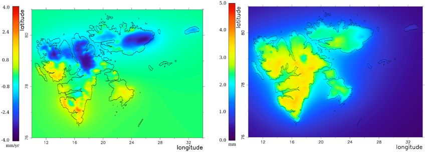
Fig. 4 illustrates the seasonal component of the loading signal at
NYALES20. A thin red line at the plot shows result of the best fit
Downloaded from https://academic.oup.com/gji/article/229/1/408/6445027 by guest on 27 February 2022
of the sinusoidal signal. However, the sinusoidal model provides a
poor fit to the data with errors reaching 40 per cent of the seasonal
signal. All constituents of this expansion for NYALES20 are shown
in Fig. 5.
In solution s3 we did not estimated annual and semi-annual si-
nusoidal variations of NYALES20 positions, but estimated admit-
tance factors for the up, east, and north components of the IAV(t) +
SEA(p(t)) mass loading time-series. In contrast to estimation of si-
nusoidal variations, the shape and phase of the signal remains fixed
when we estimate admittance. The adjusted parameter is the scaling
factor of the modeled displacement magnitude. The power of this
approach is that it allows us to evaluate quantitatively the amount
of the modeled signal in data, and test a statistical hypothesis that
all model signal is present in the data.
Figure 3. GNSS vertical time-series for the Gamit-NMA solutions. The The results of admittance factor estimation are presented in Ta-
color coded time span is the data period used in this study. The black curves ble 3 in row ADM TOT. Then we estimated the admittance factor for
are the model function fitted to this period. The HORN station was moved the seasonal SEA[p(t)] and interannual variations IAV(t) separately
to a new location in 2009. The time-series are shifted with respect to each in the s4 solution.
other to improve readability.
factor. We assume that the time-series of the displacement in ques-
tion d(t) is present in data as a · d(t) where a is a dimensionless
parameter called an admittance factor that is assumed constant for 2.5 Gravimetry/SCG
the time period of observations. The admittance factor describes We use gravity measurements from two SCG instruments cover-
what share of the modeled signal is present in observations. ing the period 1999 to 2018 to estimate gravity change. Gravity
We noticed that seasonal crustal deformations of NYALES20 measurements from 1999 to 2013 and 2014 to 2018 are collected
positions are periodic but not sinusoidal. The shape of these varia- with C039 and iGrav012 SCG instrument, respectively. The original
tions is surprisingly stable with time (Fig. 4). We decomposed the gravity measurements have a spacing of 1 second, giving a total of
mass loading signal into four components: seasonal, interannual, approximately 620 million measurements. They are resampled ev-
linear trend, and residuals. The decomposition was performed in ery minute using a symmetric numerical Finite Impulse Response
three steps. First, the mass loading time-series were filtered with (FIR) zero phase low-pass filter with a cut-off at 120 s (Wenzel
the low-pass Gaussian filter, which provided a coarse interannual 1996). Data was then cleaned for outliers and earthquakes. We cor-
signal (IAV(t)). Secondly, the time-series were folded of the phase rected for the effect of air pressure using the value of –0.422 ±
in a form p = (t − t0 )/t, where t is time, t0 is the reference epoch 0.004 μGal hPa–1 found by Sato et al. (2006a). Both the solid earth
2000.0, t is the period (1 yr), and then smoothed. That provided a and ocean tides are removed from the gravity data by estimating
coarse estimate of the seasonal signal [SEA(t), blue curve in Fig. 4]. a synthetic tide based on Hartmann & Wenzel (1995) tidal model
Then we adjusted parameters A, B, ai , si of the decomposition of the and a set of tidal parameters. The synthetic tide is estimated using
loading displacements D(t) described by the eq (4), using a single ETERNA 3.4 (Wenzel 1996).
least square solution: We also estimated and removed the instrumental drift by compar-
ing to absolute gravity measurements. We estimated a linear drift
DCMB (t) = IAV(t) + SEA( p(t)) + A + Bt + ε(t), (4)
(using unweighted least squares) by comparing to ten AG measure-
where ments (2000, 2001, 2002, 2004, 2007, 2010, twice in 2012, 2014,
2017). The estimated value is –2.74107 ± 0.17 μGal yr–1 . Finally,
IAV(t) = ai Bi (t) we re-sampled the data first every 5 min and then every 1 hr us-
i
ing a symmetric FIR zero phase filter (cut-offs 1250 s and 2 hr,
SEA(t) = si Bi ( p(t)), respectively) and then to daily values using a flat filter.
i
Seasonal glacier and snow loading in Svalbard 413
Table 2. VLBI analysis strategies.
Where pSolve
A priori radio source coordinates ICRF3 S/X Solved for
A priori EOP C04 combined Solved for
Elevation angle cut-off 0◦ 5◦
Troposphere mapping function VMF1 Direct integration
(Boehm et al. 2006) Using output of
Numerical weather
Model GEOS-FPIT
Solid Earth tide IERS2010 Elastic
(Mathews et al. 1997)
Ocean tidal loading TPXO7.2 FES2014B
Ocean pole tide IERS2010 IERS2010
Higher order ionosphere Not applied Applied
Downloaded from https://academic.oup.com/gji/article/229/1/408/6445027 by guest on 27 February 2022
Table 3. Admittance factors of NYALES20 displacements
caused by LWS loading. The first row, ADM TOT shows the ad-
mittance factor estimate from s3 solution of the total mass load-
ing signal. Rows ADM SEA and ADM IAV shows estimates of
the seasonal and interannual constituents of the loading signal
from s4 solution respectively.
Factor Up East North
ADM TOT 1.38 ± 0.04 0.62 ± 0.05 2.05 ± 0.12
ADM SEA 1.10 ± 0.05 0.47 ± 0.11 6.10 ± 0.49
ADM IAV 2.90 ± 0.07 2.44 ± 0.11 1.00 ± 0.15
2.6 Filtering of Common Mode and elastic loading signal
It is well known that stations in a region can have a spatially cor-
related signal, a so-called CM signal (Wdowinski et al. 1997), and
that removal of the CM signal can reduce noise in the time-series.
The CM signal could come from the GNSS analysis strategy and
from the strategy for reference frame realization. It could come
from mismodelled orbit, clocks or EOPs, or through unmodelled
Figure 4. Folded periodic up LWS mass loading displacements of large scale hydrology or atmospheric effects. To remove such signal
NYALES20 after removal of the slowly varying constituent. The thick blue either CM filtering, Empirical Ortoghonal Functions (EOF) or re-
line shows the estimate of the seasonal constituent. Green dots show the
gional reference frame realization, can be used. All these methods
mass loading signal after removal of the interannual constituent. A red thin
line shows a sinusoidal fit in a form a cos 2π p + b sin 2π p, where p is the
presuppose that we have stations exposed to the same undesirable
phase of the seasonal signal in turns. CM signal. In Arctic areas, we have limited access to nearby sta-
tions. All stations on Svalbard are exposed to similar signals from
glaciers, using one or several of these stations for removal of the
CM signal will not only remove the CM signal, but also the real
elastic signal from snow and ice.
The station BJOS at Bear Island is located 240 km south of
Svalbard. The Island is small and surrounded by ocean and the
local loading signal from ice and snow is approximately 10 per cent
of the signal in Ny-Ålesund (see Tabel A2). It is the closest GNSS
station outside Svalbard. Time-series of the BJOS station are used
to estimate the CM signal. Time-series for the BJOS station, and
hence CM filtering, are only included in the solutions computed by
the authors (Gamit-NMA, GipsyX-FID and GipsyX-NNR) and not
available in the external solutions (SOPAC, JPL, UNR and ITRF).
The CM filtered time-series for the ith station is then:
i
HCM (t) = HGNSS
i
(t) − CM(t) = HGNSS
i
(t) − HGNSS
BJOS
(t), (5)
i BJOS
Figure 5. Three constituents of the vertical LWS mass loading at station where t is the epoch and and
HGNSS HGNSS
is the time-series for
NYALES20. The thick blue line shows the interannual variation, the green station i and BJOS, respectively.
thin line shows the seasonal component, and red dots in the bottom shows The CM filtering removes the common error signal at the stations
the residual signal. The residual signal is artificially shifted by –8 mm. The as well as real measured signal at BJOS. If the station at Bear
linear trend is removed and not shown. Island has an unique unmodelled loading signal not present in other
Svalbard stations, this unique signal will be erroneously subtracted
also from the other stations.414 H.P. Kierulf et al.
Table 4. Trend, annual- and semi-signal in Ny-Ålesund and Bear Island. The parameters are estimated trend and annual signal
estimated using eq. (3). The results are for different GNSS solutions, VLBI, SCG and NTL in Ny-Ålesund and Bear Island. In the
VLBI time-series a pure white noise model is assumed. The gravity values (∗) are converted to millimeter using the convertion ratio
–0.24 μGal mm–1 from Mémin et al. (2012). CM is the CM filtered time-series described in Section 2.6. NTL is the sum of non tidal
elastic loading signal from ATM, NTO and LWS including the load from snow and glacier from the CMB model.
Station Trend (mm yr–1 ) Annual signal Semi-annual signal
Amp. (mm) Pha. (◦ ) Amp. (mm) Pha. (◦ )
NYA1 Gamit-SOPAC 9.61 ± 0.62 6.28 ± 0.64 –51.3 ± 5.8 1.71 ± 0.44 107.1 ± 14.6
Gamit-NMA 9.62 ± 0.62 5.80 ± 0.64 –13.0 ± 6.3 1.42 ± 0.44 57.6 ± 17.2
GipsyX-FID 9.49 ± 0.69 3.05 ± 0.70 –45.7 ± 13.0 1.05 ± 0.45 123.1 ± 23.2
GipsyX-NNR 9.26 ± 0.67 2.96 ± 0.69 –27.4 ± 13.1 0.91 ± 0.42 134.0 ± 24.8
GipsyX-UNR 9.27 ± 0.67 2.91 ± 0.69 –27.6 ± 13.3 0.91 ± 0.42 135.2 ± 24.8
GipsyX-JPL 9.59 ± 0.65 3.36 ± 0.66 –12.9 ± 11.1 1.08 ± 0.43 161.5 ± 21.9
ITRF2014 9.00 ± 0.95 4.05 ± 0.75 –36.2 ± 10.5 1.08 ± 0.47 157.5 ± 23.6
Gamit-NMA (CM) 9.55 ± 0.36 4.07 ± 0.38 –47.5 ± 5.4 0.66 ± 0.26 113.1 ± 21.3
Downloaded from https://academic.oup.com/gji/article/229/1/408/6445027 by guest on 27 February 2022
GipsyX-FID (CM) 9.80 ± 0.31 2.84 ± 0.34 –54.0 ± 6.8 0.86 ± 0.24 136.5 ± 15.9
GipsyX-NNR (CM) 9.86 ± 0.35 2.91 ± 0.38 –58.2 ± 7.4 0.82 ± 0.27 127.9 ± 18.1
NYAL Gamit-SOPAC 9.41 ± 0.61 6.24 ± 0.63 –56.6 ± 5.8 1.96 ± 0.44 105.8 ± 12.7
Gamit-NMA 9.57 ± 0.67 5.22 ± 0.69 –12.9 ± 7.6 1.75 ± 0.48 64.3 ± 15.4
GipsyX-FID 9.34 ± 0.67 3.45 ± 0.74 –59.4 ± 12.1 1.16 ± 0.48 122.1 ± 22.5
GipsyX-NNR 9.14 ± 0.66 3.19 ± 0.68 –39.9 ± 11.9 1.12 ± 0.45 124.2 ± 21.6
GipsyX-UNR 9.13 ± 0.65 3.17 ± 0.66 –39.9 ± 11.8 1.11 ± 0.44 125.5 ± 21.6
GipsyX-JPL 9.39 ± 0.65 3.44 ± 0.66 –27.7 ± 10.9 1.17 ± 0.44 153.2 ± 20.8
ITRF2014 9.34 ± 0.98 4.37 ± 0.78 –47.7 ± 10.1 1.17 ± 0.50 156.1 ± 23.0
Gamit-NMA (CM) 9.52 ± 0.35 3.60 ± 0.37 –52.9 ± 5.9 0.96 ± 0.26 102.8 ± 15.3
GipsyX-FID (CM) 9.67 ± 0.33 3.34 ± 0.38 –63.9 ± 6.5 1.17 ± 0.28 122.9 ± 13.4
GipsyX-NNR (CM) 9.75 ± 0.34 3.45 ± 0.36 –68.1 ± 6.0 1.11 ± 0.26 120.6 ± 13.4
NYALES20 Where 8.87 ± 0.17 2.62 ± 0.80 –67.3 ± 17.9 1.14 ± 0.81 77.3 ± 31.5
NYAL-SCG ∗ 2.52
± 0.64 ∗ 14.38± 0.67 –83.8 ± 2.7 ∗ 3.92
± 0.47 60.6 ± 6.8
Ny-Ålesund NTL 0.92 ± 0.30 4.00 ± 0.32 –82.5 ± 4.6 1.21 ± 0.22 111.3 ±10.3
BJOS Gamit-NMA 0.10 ± 0.54 3.30 ± 0.55 32.6 ± 9.5 1.14 ± 0.38 33.6 ± 18.4
GipsyX-FID –0.27 ± 0.62 0.90 ± 0.47 21.2 ± 27.3 0.62 ± 0.32 45.5 ± 27.5
GipsyX-NNR –0.47 ± 0.59 1.63 ± 0.58 46.1 ± 19.6 0.57 ± 0.30 –54.0 ± 27.6
Bear Island NTL –0.04 ± 0.31 1.99 ± 0.32 –107.7 ± 9.1 0.38 ± 0.18 100.1 ±25.3
To CM filter a time-series where the signal from a loading model where LIN is the linear part and ε contains the noise. The noise
is removed, the loading signal for the station(s) used in the CM includes unmodeled loadings, but also station dependent effects
filtering has to be removed as well. In our case, the loading signal like multipath, atmospheric effects, not use of individual antenna
was subtracted both for the BJOS time-series before computing calibration, and thermal expansion of antenna monument. Possible
the CM signal and for the other Svalbard time-series before the unique unmodelled signal from BJOS will also map into the noise
CM filtering. The final Svalbard time-series are cleaned for both the term. Splitting the load signal into a signal from glacier and snow,
regional CM signal over Svalbard and Bear Island and the estimated HGS , and other non-tidal loadings, HNTL∗ , we can rewrite eq. (7)
load signal. The CM filtered time-series for station i is then: into:
i
HCM,L (t) = HGNSS
i
(t) − HLi (t) − CM(t), (6) L I N i (t) + HGS
i
(t) + ε(t) = HGNSS
i
(t) − HNTL
i
∗ (t)
BJOS
i
where t is the epoch, HGNSS is the observed time-series, HLi is the − HGNSS (t) − HNTLBJOS
∗ (t)
estimated loading signal, and CM is the common mode signal. As − HGS (t) ,
BJOS
(8)
described earlier, we use the time-series from BJOS to estimate the
that is we have isolated the linear part and the elastic signal from
CM signal, but since we remove the estimated loading signal from
glaciers and snow as a sum of known terms.
the time-series, we have to remove the loading signal from BJOS
time-series before computing the CM signal. Therefore, we get
i
HCM,L (t) = HGNSS
i
(t) − HLi (t) − (HGNSS
BJOS
(t) − HLBJOS (t)). (7) 3 R E S U LT S A N D D I S C U S S I O N
The vertical component of the different GNSS solutions in Ny-
Ålesund and Bear Island as well as the NTL signal are included
2.7 Isolating the elastic signal from glacier and snow
in Table 4. In addition, the Where results (Solution s1) from the
The signal in HCM, L (t) (eq. 7) includes all vertical motions not NYALES20 VLBI antenna and the SCG in Ny-Ålesund are in-
accounted for in the loading models or CM filtering, for example cluded. Some of the time-series are plotted in Fig. 6. The horizontal
unmodelled loading, Glacial Isostatic Adjustment (GIA), tectonics, components of the different GNSS solutions are included in Ta-
and noise. Assuming that the GIA and the tectonic component are ble A1. The loading signals for all the different loading models are
linear, the left hand side can be written HCM, L (t) = LIN(t) + ε(t), included in Table A2.Seasonal glacier and snow loading in Svalbard 415
Downloaded from https://academic.oup.com/gji/article/229/1/408/6445027 by guest on 27 February 2022
Figure 6. A selected set of detrended time-series for Svalbard. The time-series are: GipsyX-NNR for NYA1 (upper left-hand panel), NTL (ATM, NTO, LWS
including the glaciers and snow) signal in Ny-Ålesund (middle left-hand panel), the GipsyX-NNR time-series for NYA1 after removal of NTL and CM filtering
(lower left-hand panel), GipsyX-NNR for BJOS (upper right-hand panel), gravity from the SCG in Ny-Ålesund (middle right-hand panel) and the NYALES20
Where solution (lower right-hand panel). The gravity values are converted to millimeter using the convertion ratio –0.24 μGal mm–1 (Mémin et al. 2012).
Figure 7. Seasonal signal in Ny-Ålesund (NYA1). The left-hand panel shows the sum of the annual and semi-annual sinusoidal signal for the time-series, the
right-hand panel shows the same results relative to the NTL signal (ATM, NTO, LWS including the glaciers and snow). The upper most five curves are from
time-series analysis of the raw time-series. The sixth and seventh curves are CM-filtered time-series. The bottom curve of the left panel is the estimated NTL
signal. The curves are shifted with respect to each other to improve readability.
3.1 Determination of the loading annual signal ITRF2014 time-series that ended in 2014. The estimated uplift for
the Ny-Ålesund stations agree below the uncertainty level.
As shown in Kierulf et al. (2009b) the uplift in Ny-Ålesund varies
The annual signal in Ny-Ålesund varies between the solutions
from year to year. Consequently, trends from different time periods
both in phase and amplitude (Table 4, Table A1 and Fig. 7). This
can not be compared directly. We have chosen to use the time
implies that the choice of GNSS analysis strategy has a noticeable
interval 2010 until 2018 for time-series analysis, except for the
impact on the estimated seasonal variations. Martens et al. (2020)416 H.P. Kierulf et al.
Table 5. Admittance factors for the vertical com- 3.2 Determination of the loading admittance factors
ponent of GNSS station in Svalbard caused by
the glacier and snow loading. ADM SEA and We found the admittance factor from VLBI solutions for the sea-
ADM IAV show estimates of the seasonal and in- sonal vertical displacement does not deviate from 1.0 at a 2σ level,
terannual admittance factors. that is the LWS signal is fully recovered from the data. At the same
time the departure of the admittance factor from 1.0 for the hori-
Station ADM SEA ADM IAV
zontal loading components implies there is a statically significant
SVES 0.94 ± 0.15 0.04 ± 0.13 discrepancy between the computed loading signal and the data. It
NYAL 1.33 ± 0.18 0.03 ± 0.17 should be noted that the magnitude of the seasonal signal in North
NYA1 1.01 ± 0.18 0.19 ± 0.16
direction is only 0.15 mm and the signal itself is just too small to
LYRS 0.95 ± 0.18 –0.11 ± 0.21
be detected. The admittance factor for the interannual signal is sig-
HORN 1.35 ± 0.16 0.25 ± 0.17
All 1.12 ± 0.07 0.11 ± 0.07 nificantly different from 1.0, which indicates that the loading signal
alone cannot explain it.
We made an additional analysis to find the admittance factor
for the glacier and snow loading signal at the GNSS stations in
found similar differences in the estimated annual signal when they
Svalbard. We computed mass loading for all the GNSS stations
Downloaded from https://academic.oup.com/gji/article/229/1/408/6445027 by guest on 27 February 2022
compared GNSS time-series, in United States and Alaska, based on
in Svalbard and fitted it to the GNSS time-series using reciprocal
different analysis strategies. Such variations make direct geophysi-
formal uncertainties as weights. Then we computed the χ 2 per
cal interpretation of the periodicity in GNSS time-series difficult.
degree of freedom of the fit and scaled variances of admittance
The measured vertical annual signal (Table 4) is smaller than
factor estimates by this amount. Table 5 shows the estimates of
the estimated NTL signal for the GipsyX solutions and larger than
the admittance factor from the differenced GNSS time-series using
the estimated NTL signal for the Gamit solutions. The phase of the
eq. (8). Similar to the VLBI case, the admittance is very close to 1.0
GNSS solutions are delayed relative to the NTL signal with between
for the vertical seasonal signal (row ‘All’) and it is far away from
30◦ and 70◦ (corresponding to a delay between 1 and 2.5 months)
1.0 for the interannual signal and the horizontal signal.
in Ny-Ålesund.
Two factors may cause poor modeling of the interannual signal.
The CM-filtered solutions are closer to the expected signal from
First, calving and frontal ablation are not included in the CMB
NTL and we have less differences between the GipsyX and Gamit
model, and therefore, lacks this contribution. Secondly, other load-
solutions (see Fig. 7). The annual signal found with the Where
ings, for instance non-tidal ocean loading may contribute. The sea-
software for VLBI has a smaller amplitude, but the phase is close
sonal signal has a very specific time dependence pattern, and the
to the phase estimated from the loading modeling.
approach of admittance factor estimation exploits the uniqueness
The phase of the gravity signal in Ny-Ålesund is close to the
of this pattern, while the pattern of the interannual signal is more
phase of the loading models. The annual amplitude in gravity is
general.
3.45 μGal. For a spherical and compressible Earth model the elastic
The analysis of the admittance factors give several important
gravity variations can be converted to vertical position variations
results in addition to the very good agreement between the different
using a ratio of –0.24 μGal mm–1 (Mémin et al. 2012). Using
estimated vertical seasonal components. Analysis of observations
this ratio we got an yearly amplitude of 14.4 mm. This is much
shows that the CMB model provides prediction of the vertical mass
larger than the estimated annual loading signal of around 4.0 mm
loading with 1σ errors of 5 per cent, which corresponds to 0.1 mm.
in Ny-Ålesund. However, the gravity variations also depends on the
We have a bias wrt to the model of 0.2 ± 0.1 mm, and this bias is not
direct gravitational attraction. Mémin et al. (2012) discussed how
statistically significant at a 95 per cent level (2σ ). We conclude that
the location of the load affect the ratio between gravity and uplift.
analysis of the data from two totally independent techniques, VLBI
Both the distance to and the relative height of the load have an
and GNSS, proves there is no statistically significant deviation at
impact. The large annual signal implies mass changes at locations
a 95 per cent significance level between the seasonal vertical mass
with negative relative heights close to the station.
loading signal based on the CMB model and observations of both
The SCG-instrument in Ny-Ålesund gives a combined signal
techniques.
from three glacier related factors. The viscoelastic response from
past ice mass changes, the immediate elastic response of the ongoing
ice mass changes, and the direct gravitational attraction from the
3.3 Geodynamic interpretation
ongoing ice mass changes on the glaciers (see Mémin et al. 2014;
Breili et al. 2017). The two latter have a clear influence on the annual To study the time-series ability to capture the loading signal from
signal. In addition, soil moisture and accumulated snow close to and glaciers and snowpack changes, we used the CM filtered time-
mainly below the gravimeter, have a much stronger effect on gravity series. Other known loading signals were removed using eq. (8).
than on displacements. To have more robust time-series, in the following discussion, we
Quantifying the gravity signal from these nearby hydrological have used averaged GNSS time-series. The averaged time-series are
factors are demanding and out of the scope of this paper. However, the weighted mean of the daily values from the Gamit-NMA, the
they, as well as glaciers, are forced by temperature and precipita- GipsyX-NNR and the GipsyX-FID solutions. The annual periodic
tion. We assume that they are in phase with the elastic uplift signal. signal and the linear rate for the time-series in eq. (8) are included
A gravimeter measures gravity changes directly, while VLBI and in Table 6 together with the elastic signal from glaciers and snow.
GNSS evaluate site positions from analysis of observations at a net- Detailed results for the individual GNSS solutions are included in
work, and a position estimate of a given station in general depends Table A3.
on measurements at other stations of the network. The phase of the The amplitudes of the estimated loading signal from glaciers
SCG time-series is therefore an independent measure of the varia- and snowpack vary with latitude and longitude and depend on the
tions in Ny-Ålesund and the result coincides with the results from amount of surrounding glaciers and land masses (see Fig. 9). The
the other techniques. station HAGN in the middle of the glacier Kongsvegen has theSeasonal glacier and snow loading in Svalbard 417
Table 6. Vertical rate and annual signal for GNSS stations in Svalbard. GS are the elastic loading signal
from ice and snow. GNSS-CM is the time-series using eq. (8). Max uplift is the date of the maximum value
for the annual signal.
Max uplift
Station Trend (mm yr–1 ) Amp. (mm) Pha. (◦ ) (date)
Up:
NYA1 GNSS-CML 9.74 ± 0.27 3.37 ± 0.29 –56.5 ± 5.0 3 Nov.
GS 0.93 ± 0.03 2.66 ± 0.03 –81.8 ± 0.6 9 Oct.
NYAL GNSS-CML 9.57 ± 0.27 3.63 ± 0.29 –67.9 ± 4.6 23 Oct.
GS 0.93 ± 0.03 2.66 ± 0.03 –81.8 ± 0.6 9 Oct.
HAGN GNSS-CML 11.95 ± 0.56 4.28 ± 0.65 –50.2 ± 8.6 10 Nov.
GS 1.81 ± 0.04 3.73 ± 0.04 –80.1 ± 0.7 10 Oct.
LYRS GNSS-CML 8.16 ± 0.42 3.21 ± 0.45 –80.8 ± 8.0 10 Oct.
GS 0.83 ± 0.03 3.21 ± 0.03 –83.2 ± 0.6 7 Oct.
SVES GNSS-CML 6.21 ± 0.45 3.37 ± 0.47 –96.8 ± 7.9 23 Sep.
GS 0.86 ± 0.04 3.53 ± 0.04 –81.9 ± 0.6 8 Oct.
Downloaded from https://academic.oup.com/gji/article/229/1/408/6445027 by guest on 27 February 2022
HORN GNSS-CML 9.45 ± 0.27 3.21 ± 0.30 –60.0 ± 5.3 31 Oct.
GS 1.93 ± 0.03 2.69 ± 0.03 –77.0 ± 0.6 13 Oct.
North:
NYA1 GNSS-CML 14.98 ± 0.09 0.24 ± 0.09 39.6 ± 21.1 9 Feb.
GS 0.56 ± 0.01 0.17 ± 0.01 –72.0 ± 1.0 18 Oct.
NYAL GNSS-CML 14.84 ± 0.12 0.47 ± 0.12 –89.5 ± 14.9 1 Oct.
GS 0.56 ± 0.01 0.17 ± 0.01 –72.0 ± 1.0 18 Oct.
HAGN GNSS-CML 14.73 ± 0.36 0.83 ± 0.34 147.7 ± 22.2 29 May.
GS 0.53 ± 0.01 0.05 ± 0.01 –49.1 ± 3.4 11 Nov.
LYRS GNSS-CML 14.47 ± 0.16 1.19 ± 0.17 63.6 ± 8.2 5 Mar.
GS 0.24 ± 0.01 0.06 ± 0.01 84.4 ± 3.6 26 Mar.
SVES GNSS-CML 14.49 ± 0.33 2.55 ± 0.33 35.4 ± 7.3 4 Feb.
GS 0.19 ± 0.01 0.24 ± 0.01 89.0 ± 1.2 31 Mar.
HORN GNSS-CML 13.20 ± 0.14 1.02 ± 0.14 91.7 ± 8.0 2 Apr.
GS –0.43 ± 0.01 0.73 ± 0.01 101.6 ± 0.7 13 Apr.
East:
NYA1 GNSS-CML 10.24 ± 0.08 0.42 ± 0.09 18.6 ± 11.8 18 Jan.
GS –0.07 ± 0.01 0.64 ± 0.01 98.3 ± 0.8 9 Apr.
NYAL GNSS-CML 10.01 ± 0.08 0.16 ± 0.07 –59.1 ± 25.0 1 Nov.
GS –0.07 ± 0.01 0.64 ± 0.01 98.3 ± 0.8 9 Apr.
HAGN GNSS-CML 12.65 ± 0.32 0.66 ± 0.29 151.4 ± 23.9 2 Jun.
GS 0.32 ± 0.01 0.40 ± 0.01 94.5 ± 0.9 5 Apr.
LYRS GNSS-CML 12.48 ± 0.17 0.35 ± 0.15 77.7 ± 23.5 19 Mar.
GS 0.08 ± 0.01 0.27 ± 0.01 95.9 ± 1.1 7 Apr.
SVES GNSS-CML 15.71 ± 0.27 0.76 ± 0.26 31.9 ± 18.8 1 Feb.
GS –0.17 ± 0.01 0.07 ± 0.01 117.7 ± 2.5 29 Apr.
HORN GNSS-CML 11.56 ± 0.11 0.45 ± 0.11 51.2 ± 13.8 20 Feb.
GS –0.31 ± 0.01 0.32 ± 0.01 106.4 ± 0.9 17 Apr.
largest estimated annual loading signal, while the westernmost sta- explain a higher observed amplitude in areas like Ny-Ålesund and
tions NYAL/NYA1 and HORN have the smallest. The GNSS sta- Hornsund, which have a lot of nearby large calving glaciers. How-
tions SVES and LYRS are located in central parts of Svalbard and ever, the deviation of admittance factors from 1.0 for these stations
here the measured vertical annual signal agrees with the estimated is still within 2σ of the statistical uncertainty. Longer time-series
loading signal at the uncertainty level. For the stations closest to the are needed to establish whether there is a statistically significant de-
west coast NYAL, NYA1 and HORN the measured amplitudes are viation of observations from the model for these individual stations.
slightly larger than expected from the variations in glaciers and snow The phase of the vertical loading signal from glaciers and snow
(∼0.7, ∼1.0 and ∼0.5 mm, respectively). Although the admittance varies with only a few days over Svalbard, and corresponds to a
factor for all stations combined show very good agreement for the maximal value after the end of the melting season, in mid-October.
seasonal component, the admittance factor for individual stations The phase of the GNSS time-series agrees with the glaciers and
in Ny-Ålesund and Hornsund are slightly above one, implying that snow signal from the CMB models within a few weeks.
the observed amplitude is somewhat larger than the prediction from The predicted horizontal seasonal signal is smaller. It is around
the CMB model. 0.2 mm in the north component for all locations except HORN.
The larger vertical amplitude at NYAL, NYA1 and HORN might HORN is located in the south of Svalbard with the majority of
be due to lower precision of the CMB models in areas with more glaciers located to the north. Consequently the north amplitude is
variable coastal climate, changes in groundwater and surface hydrol- larger, 0.7 mm. The other stations have glaciers both to the north
ogy, and seasonal variability in calving/frontal ablation of glaciers. and to the south and the loading signals are cancelled out. The
Especially, calving is assumed to be seasonally dependent with east annual signal varies from 0.7 mm (NYAL, NYA1) to 0.0 mm
higher incidents during summer (when ice flows faster). This may (SVES), depending on their locations relative to the glaciers.418 H.P. Kierulf et al.
Our CMB model is limited by Svalbard archipelago. Glacial
loading at other islands, such as Iceland and Greenland, can bring a
noticeable contribution (Kierulf et al. 2021, Coulson et al. 2021).
Using Green’s function from the ocean tide loading provide of Sch-
erneck (1991),1 assuming 100 Gt seasonal ice cycle on Greenland
(see Fig. 6 in Bevis et al. 2012), and the average distance from
Greenland to Svalbard of 800 km, we get coarse estimate of the
the amplitude of mass loading signal Svalbard due to glacier in
Greenland: 0.38 mm. In order to get a more refined estimate of the
magnitude of such a contribution, we used Loomis et al. (2019)
mascon solution for Greenland for 2008 from processing GRACE
mission. The mascon for Greenland at a regular grid 0.5◦ × 0.5◦ is
provided2 with a monthly resolution in the height of the column of
water equivalent that covers the entire land and is zero otherwise.
The mascon excludes the contribution of the atmosphere and ocean
Downloaded from https://academic.oup.com/gji/article/229/1/408/6445027 by guest on 27 February 2022
Figure 8. The seasonal contribution of glaciers in Greenland to the vertical
but retains the contribution of land water, snow, and ice storage.
displacement of NYALES20 after removal of the slowly varying constituent We have converted the height of the column of water equivalent to
from processing GRACE data. The green line shows the total contribution, surface pressure and computed the mass loading from the mascon
the shadowed blue line shows the residual contribution after subtraction of using the same approach as we used for computing atmospheric
land water storage pressure from MERRA2 model. The horizontal axis is a and land water storage loading using spherical harmonic transform
phase of the seasonal signal in phase turns. of degree/order 2699. Since MERRA2 land water storage model
covers Greenland, we computed mass loading two times: the first
time using the total surface pressure from the mascon and the second
time after subtracting the pressure anomaly from MERRA2. In the
latter case the resulting mass loading signal provides a correction
to the mass loading from MERRA2 model for the contribution of
glacier derived from GRACE data analysis since MERRA2 has
large errors of modeling glacier dynamics. The results are shown in
Fig. 8 after removal linear trend. The residual signal has amplitude
0.15 mm and is in phase with the mass loading signal from Svalbard
glacier while the total signal has amplitude 0.28 mm. This estimate
agrees remarkably well with our coarse estimate. Accounting for the
contribution of glacier mass loading using GRACE data reduces
the admittance factor from 1.10 to 1.04 for the seasonal vertical
component of the VLBI solution.
We exercise a caution in results of processing GRACE data, A
thorough analysis of systematic errors of mass loading signal from
GRACE mascon solution requires significant efforts and is beyond
the scope of the present manuscript. However, our estimates shows
that the contribution of glaciers in Greenland is not dominated and
its accounting improves the agreement of the CMB model with
VLBI and GNSS observations.
3.4 CMB model and time-series
In the previous section we examined how the different GNSS time-
series were able to capture the elastic loading signal from local
Figure 9. Annual signal for GNSS stations in Svalbard. The bars are the ice and snow changes. In this paragraph we will discuss the ef-
amplitude and the vectors are the phase. Blue is from the loading prediction fect of removing the loading signal from the time-series, both on
from glaciers and snow red is from the GNSS stations. the unfiltered time-series and the CM filtered time-series. We will
in particular look at the effect of replacing the global hydrologi-
We see that the estimated annual signal for the GNSS stations cal model with a regional CMB model. In the discussion we used
NYA1, HAGN, LYRS and HORN agree at 2σ level in the east com- an averaged time-series from the GNSS solutions; Gamit-NMA,
ponent. HORN is capturing the larger north annual signal for this GipsyX-FID and GipsyX-NNR. Due to limited observations during
location. However, the small north signals for the other stations are winter the HAGN time-series are not directly comparable with the
too small to be detected. LYRS and SVES have a large north annual other time-series and therefore not included in this discussion.
signal, 1.1 mm resp. 2.3 mm larger than expected loading signal. We
have not established the origin of this discrepancies. Possible rea-
sons are uneven thermal expansion of the antenna monument (steel
mast) and artefacts of the atmosphere model. We will investigate 1 Fig. 2 in http://holt.oso.chalmers.se/loading/loadingprimer.html
these signals in the future. 2 Available at https://earth.gsfc.nasa.gov/geo/data/grace-masconsYou can also read