ROV assessment of mesophotic fish and associated habitats across the continental shelf of the Amathole region
←
→
Page content transcription
If your browser does not render page correctly, please read the page content below
www.nature.com/scientificreports
OPEN ROV assessment of mesophotic
fish and associated habitats
across the continental shelf
of the Amathole region
Rio E. Button1*, Denham Parker1,2, Vivienne Coetzee1, Toufiek Samaai1,2,3, Ryan M. Palmer4,
Kerry Sink5,6 & Sven E. Kerwath1,2
Understanding how fish associate with habitats across marine landscapes is crucial to developing
effective marine spatial planning (MSP) in an expanding and diversifying ocean economy. Globally,
anthropogenic pressures impact the barely understood temperate mesophotic ecosystems and South
Africa’s remote Amathole shelf is no exception. The Kei and East London region encompass three
coastal marine protected areas (MPAs), two of which were recently extended to the shelf-edge. The
strong Agulhas current (exceeding 3 m/s), which runs along the narrow shelf exacerbates sampling
challenges. For the first time, a remotely operated vehicle (ROV) surveyed fish and their associated
habitats across the shelf. Results indicated fish assemblages differed between the two principle
sampling areas, and across the shelf. The number of distinct fish assemblages was higher inshore and
on the shelf-edge, relative to the mid-shelf. However, the mid-shelf had the highest species richness.
Unique visuals of rare Rhinobatos ocellatus (Speckled guitarfish) and shoaling Polyprion americanus
(wreckfish) were collected. Visual evidence of rhodolith beds, deep-water lace corals and critically
endangered endemic seabreams were ecologically important observations. The ROV enabled in situ
sampling without damaging sensitive habitats or extracting fish. This study provided information
that supported the Amathole MPA expansions, which extended protection from the coast to beyond
the shelf-edge and will guide their management. The data gathered provides baseline information for
future benthopelagic fish and habitat monitoring in these new MPAs.
Understanding how fish associate with habitats across marine landscapes is crucial to developing effective con-
servation and sustainability strategies1. If fish assemblages are associated with specific habitats and environmental
features, then this information can be used for fish distribution p rojections2. This understanding is valuable for
marine spatial planning (MSP), where information from different models can help strategize to mitigate the
effects of anthropogenic pressures3. Anthropogenic pressures are rapidly altering marine ecosystems, including
the scarcely understood mesophotic (between 30 and 150 m deep)4 and the ‘rariphotic’ (150–300 m depth) z one5.
Examples of these pressures include fishing, ocean warming, acidification and p ollution6. There is some evidence
that the mesophotic zone provides refugia from these pressures in the tropics7 however, there is no comparable
support in temperate zones8 where mesophotic biotic surveys are generally rare9.
Access to sampling the mesophotic zone is increasing as technological underwater video techniques advance10.
Previously, visual biotic surveys were focused within regular scuba depths (typically up to 30 m) and more
expensive techniques such as using submersibles focused on the deep sea4. With the development of Remotely
Operated Vehicles (ROVs), submersibles and Autonomous Underwater Vehicles, non-destructive video sampling
can be conducted across the mesophotic z one11. Some fish and mobile invertebrate species may actively avoid
ROVs, which can compromise taxonomic resolution from underwater video s urveys12. Despite these limitations,
ROV videos provide a permanent record of fish abundance, composition and associated h abitat13, allowing for
1
Department of Biological Sciences, University of Cape Town, Rondebosch 7700, South Africa. 2Department
of Forestry, Fisheries and the Environment, Cape Town 8000, South Africa. 3Department of Biodiversity and
Conservation, University of the Western Cape, Bellville, Cape Town, South Africa. 4South African Institute for
Aquatic Biodiversity, Somerset Street, Makhanda 6139, South Africa. 5South African National Biodiversity
Institute, Rhodes Drive, Newlands 7700, South Africa. 6Institute for Coastal and Marine Research, Nelson Mandela
University, Summerstrand, Gqeberha 6001, South Africa. *email: riobutton@gmail.com
Scientific Reports | (2021) 11:18171 | https://doi.org/10.1038/s41598-021-97369-2 1
Vol.:(0123456789)
www.nature.com/scientificreports/
Figure 1. Study area, the Amathole continental shelf, on the south coast of South Africa where the East London
(triangles) and Kei (squares) sampling sites were located. The 50 m bathymetric depth contours; existing MPAs,
which were declared as official reserves in 1984 and later proclaimed as MPAs in 2011; and the new MPAs,
proclaimed in 2019 are indicated. The MPAs are divided into zones with different restrictions namely (1)
no-take; (2) controlled fishing, where extraction and harvesting of marine life is allowed with restrictions and
limitations; and (3) controlled pelagic fishing, where only pelagic linefishing of specific species is permitted. Map
created in QGIS ver. 3.8 (https://qgis.org/en/site/56) using shapefiles provided by the South African National
Biodiversity Institute (https://www.sanbi.org/64) and sampling sites locations generated by this study.
a better understanding of the distribution of fish and habitat through the mesophotic zone10,14 without caus-
ing damage to the habitat or extracting s pecies15. This makes it an ideal method for sampling areas of potential
conservation value or protected areas15.
There is a global commitment to increasing marine protected area (MPA) c overage16. In 2019, South Africa
expanded MPA coverage from 0.4 to 5% of its Exclusive Economic Zone by increasing the number of MPAs
from 21 to 4117. The new MPAs are focused on offshore protection18 and aim to be representative of offshore
ecosystems and mitigate pressures from government planned ocean economy growth and industrialisation19.
The new MPAs include the offshore expansion of existing MPAs. The Amathole region on the East coast of
South Africa is considered an endemism hotspot20 and these areas were made reserves in 1984 and later MPAs
in 201121. The new Amathole Offshore MPA extends protection to the mesophotic ecosystems in the region for
the first t ime22 (Fig. 1).
The Amathole region is a transition zone between two of the six defined marine Ecoregions of South Africa:
the Agulhas (South Coast) and Natal (East Coast) E coregions18. The Agulhas Ecoregion is characterised by
warm temperate waters, the widest margin of the country’s continental shelf (up to 240 km) and several reef
complexes that hold the highest number of the country’s endemic fish species15. Distinguishing features of the
Natal Ecoregion include subtropical waters, a narrow continental shelf (5–50 km), high riverine input, steep
shelf-edges with numerous incising canyons, complex oceanographic patterns (upwelling cells and cyclonic
eddies) driven by the dominant Agulhas current15. Apart from our surveys, which were prioritised to inform
MPA placement prior to increasing coverage in 2 01917, the area is largely unexplored as it has treacherous sea
conditions. Strong currents persist throughout the area due to the Agulhas current being funnelled nearshore
by the narrow continental s helf23. Furthermore, increased regulation on fisheries, particularly the commercial
epletion24,25 resulted in a substantial decrease in commercial fishing effort in the
linefish sector, in response to d
Amathole area over the past two decades26,27. Subsequently, commercial landings data have decreased to such
Scientific Reports | (2021) 11:18171 | https://doi.org/10.1038/s41598-021-97369-2 2
Vol:.(1234567890)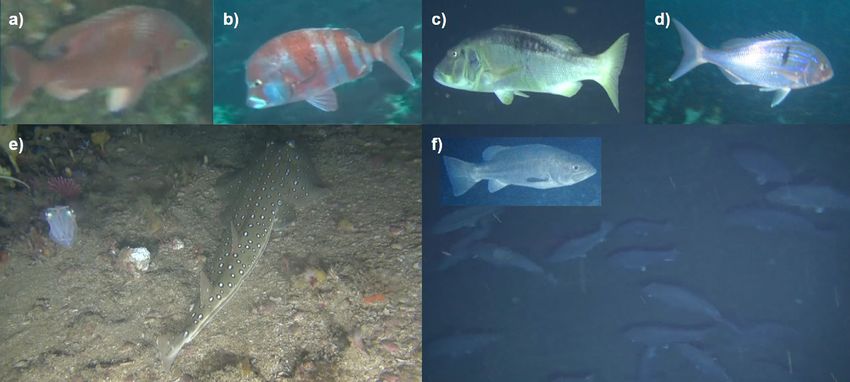
www.nature.com/scientificreports/
Figure 2. Fish images extracted from the ROV transect videos. Fish species that were endemic to South
Africa include (a) Chrysoblephus cristiceps (dageraad) (critically endangered), (b) Chrysoblephus gibbiceps
(red stumpnose) (endangered), and (c) Petrus rupestris (red steenbras) (endangered). While (d) Polysteganus
undulosus (seventy-four) was critically endangered and endemic to southern Africa. A living (e) Rhinobatos
ocellatus (speckled guitarfish) and shoaling (f) Polyprion americanus (wreckfish) were recorded on video for the
first time.
an extent that it is no longer a reliable source of information on fish distribution and abundance in the area, and
alternative data collection methods are required.
The aim was to visually explore and describe fish fauna and their associated benthic habitat as well as to
determine which environmental variables (benthic biotic, substrate, and relief habitat variables as well as depth,
distance from shore, and principal sampling areas) best explain patterns of fish distribution, abundance, and
assemblage composition. To survey benthopelagic fish and their associated habitat, an ROV ran transects. We
quantitatively surveyed fish species diversity and relative abundance in relation to depth, distance from shore
and benthic habitat to provide a baseline assessment and assess the potential of ROVs as a sampling tool in a
region characterised by strong currents. The study also represents the first visual survey of the capture site of
the first coelacanth28. The outcomes of this study are aimed to support and guide marine spatial planning and
conservation in the region.
Results
A total of 54 h of footage was collected from 42 ROV transect dives (Supplementary Table S1) which translates
to a total of 117 sampling sites (see “Methods” for how sampling sites were determined). From the 1829 MaxN
observations made, a total of 65 fish species from 49 genera and 31 families were recorded (Supplementary
Table S2), and 98% of observed fish were able to be identified to species level.
Eight morphospecies groups were identified as taxonomic species names could not be determined for these
groups. There was not enough visual detail in the footage to discern the specific species from their close relatives
(e.g., members of Congridae). Interestingly, the morphospecies ‘lab suez’ was likely a species from the genus
Liopropoma, which taxonomic experts hypothesised was a yet to be described species or species morph. In these
cases, the species were given a unique identifier. The smallest fish species we were able to reliably identify was ~8
cm, was a Nemanthias carberryi (threadfin goldie). In all but one instance, it was possible to identify the families
to which the morphospecies belonged. Of the species observed 32 were endemic to southern Africa and 14 to
South Africa. Species diversity per sample site ranged from 0 to 19, average species richness (± standard devia-
tion (s.d)) was 5.70 (± 4.28) and mean total species abundance (± s.d.) was 15.63 (± 16.28). The most frequently
observed families were Sparidae (17 spp.), Serranidae (7 spp.), Labridae (4 spp.), and Triglidae (1 spp.) (Supple-
mentary Table S2). The ROV allowed us to observe rare large, overexploited and critically endangered endemic
seabreams including Polysteganus undulosus (Seventy-four) and Chrysoblephus cristiceps (Dageraad) as well as
endangered Chrysoblephus gibbiceps (Red stumpnose) and Petrus rupestris (Red steenbras)24,25 (see Fig. 2a–d).
Three endangered Sphyrna lewini (Scalloped hammerhead) were observed on a single transect that had a median
depth of 90m. This study collected unprecedented observations of Polyprion americanus (Wreckfish) schooling
as well as Rhinobatos ocellatus (Speckled guitarfish), which were both listed as data deficient by the IUCN red
list30 (Fig. 2e,f). Rare habitat types, including rhodolith beds, sponges, and deep-water lace corals were also
documented (Fig.3 and Supplementary Table S3).
The number of unique habitat variables observed included 12 substrata, 25 benthic biotas, and 4 reliefs (Sup-
plementary Table S3). The most abundant substrate observed was rock (43%), the most abundant benthic biota
was fan coral (soft coral) (23%), and ‘flat’ (48%) was the most abundant form of relief. Rhodolith substrate was
Scientific Reports | (2021) 11:18171 | https://doi.org/10.1038/s41598-021-97369-2 3
Vol.:(0123456789)www.nature.com/scientificreports/
Figure 3. Images of dominant habitat for substrate clusters: (a) sand, (b) rubble, (c) rhodoliths and (d) rock.
Biota clusters included: (e) no biota, (f) algae, (g) soft corals & sponges and (h) fan coral; and relief clusters (i)
flat and (j) low, were extracted from the ROV transect videos.
documented between 33 and 64 m deep, with individual agglomerates being approximately 3–12 cm in diameter.
Encrusting coralline algae were observed to a depth of 80 m. This was the deepest photosynthesising organism
observed, which may be an indication of the maximum depth to which photosynthesis occurs in the region.
Notable biotic habitats frequently observed included deepwater lace coral and sponge gardens. Habitat clustered
into four substrate clusters, four biotic clusters and two relief clusters. Substrate clusters were dominated by sand,
rhodoliths, rubble (coarse biogenic rubble), and rock respectively. No specific biota type dominated the benthic
biota clusters, but lace corals, sponges, algae and sea fans were abundant at various depths while the relief clusters
were dominated by flat and low relief (Fig. 3 and Supplementary Table S4).
Mean (± s.d) of species diversity was similar for the Kei and East London areas, 49 (± 0.43) and 47 (± 0.45),
respectively. The important predictor variables for fish abundance data (in descending order) were substrate,
distance from shore, depth, and principal sampling area (Kei and East London). These variables were included
in the Multivariate Regression Tree (MRT) which resulted in the formation of ten unique fish assemblages. The
fish assemblages initial split was explained by depth, the split occurred at 94 m (Supplementary Fig. S2). Species
composition overlapped between assemblages (Supplementary Fig. S3). Assemblages were patchily distributed,
however, similar assemblages tended to occur spatially close together—there were four fish assemblages unique
to East London while one was unique to Kei (Fig. 4). Fish assemblages also varied along the shelf gradient, with
higher fish assemblage diversity on the inshore and shelf-edge relative to the mid-shelf. Mean (± s.d.) species
richness inshore (100 m depth) was 17 (± 0.44). When species
richness was examined, distance from shore and depth were found to be co-linear, but the former was the better
predictor of species richness. With distance from shore as a predictive variable, species richness peaked in the
middle of the continental shelf (approx. 12 km from the shore). Species richness declined linearly with increasing
depth. Substrate was the only significant variable for predicting species richness, and higher species richness was
associated with consolidated substrates, rhodolith and rock (Fig. 5 and Supplementary Table S4). Substrate was
the most important benthic habitat predictor for three of the five most abundant species: Cheilodactylus pixi,
Chirodactylus brachydactylus and Chelidonichthys capensis. The formers abundance was associated with rubble
while the abundance of the latter two was associated with rhodoliths. Of the remaining two species, Serranus
knysnaensis abundance peaked in fan coral biota and Pterogymnus laniarius was most frequently observed in
low relief areas (Fig. 6 and Supplementary Table S5).
Discussion
With the use of ROVs, this exploratory study provided the first assessment of deeper mesophotic reefs, their
benthopelagic ichthyofaunal assemblages and associated benthic habitats in the Amathole region of South Africa.
This environment was previously inaccessible to scientific surveys. This study revealed an abundance of seabream
(Family: Sparidae) species including Polysteganus undulosus, Chrysoblephus gibbiceps, Pterogymnus laniarius, and
Argyrozona argyrozona. Their abundance is most encouraging as in 2000 South Africa’s traditional linefishery
was declared in a state of emergency and the urgent need to rebuild the many overexploited linefish stocks was
recognised29,31. After this species-specific management plans began being drawn up and were implemented in
the mid-2000’s29,31. Study highlights included the first footage of Rhinobatos ocellatus, as well as the shoaling
behaviour of Polyprion americanus—both species were classified as data deficient by the IUCN r edlist28. Rhinoba-
tos ocellatus was only known from three bycatch s pecimens32, despite their distinctive appearance32,33. Typically,
Polyprion americanus was solitary and only known to aggregate off the coast of Brazil to spawn34. Their shoaling
on the Amathole shelf-edge above deep-water corals suggests that the area might be a spawning habitat for this
Scientific Reports | (2021) 11:18171 | https://doi.org/10.1038/s41598-021-97369-2 4
Vol:.(1234567890)www.nature.com/scientificreports/
Figure 4. Spatial distributions of the fish assemblages on the Amathole continental shelf, located on the south
coast of South Africa. Fish assemblages are clusters of species determined using a Multivariate Regression Tree
that includes depth, substrate clusters, distance from shore and the two broad areas of East London and Kei.
These fish assemblages are labelled 1 to 10. The 50 m bathymetric contours as well as existing and new Marine
Protected Areas (MPAs) are indicated. The existing MPAs were declared as official reserves in 1984 and later
proclaimed as MPAs in 2011 and the new MPAs were proclaimed in 2019. The MPAs are divided into zones with
different restrictions namely (1) no-take, (2) controlled fishing, where extraction and harvesting of marine life
are allowed with restrictions and limitations, and (3) controlled pelagic fishing, where only pelagic linefishing
of specific species may occur. Map created in QGIS ver. 3.856 using shapefiles provided by the South African
National Biodiversity I nstitute64 and fish assemblages generated in R statistical s oftware59(CRAN ver. 4.0.2).
species; deep-water coral habitats are known to provide nurseries and spawning grounds for many species35. The
benthic habitats sampled across the Amathole shelf were generally diverse and sometimes patchy in distribution.
iodiversity36.
These findings contribute to the little that is known about South Africa’s offshore continental shelf b
The most important predictor of the five most abundant fish species differed, only Chirodactylus brachydac-
tylus and Chelidonichthys capensis had their most important predictor in common, which was distance from
shore. Hard substrate was an important predictor for Cheilodactylus pixi, Chirodactylus brachydactylus, and
Chelidonichthys capensis, the latter two species were associated with rhodoliths while the former was associate
with rubble. Substrate influences the seabed relief as well as the biota that can grow in a particular area, which
could explain the relative importance of this variable. Biota was the most important predictor of Serranus knys-
naensis abundance, which is a sedentary s pecies37 and was commonly observed sheltering from strong currents
behind fan corals. This observation was further justified with fan coral habitats having the highest MaxN for this
species. Soft corals such as fan coral have been shown to provide shelter, a source of food or a surface on which
epiphytic food was sourced38. Lastly, relief was the most important predictor for Pterogymnus laniarius. Low
relief increased the probability of the species presence which aligns with the findings that Pterogymnus laniarius
feed in sand and mud habitats as their stomach contents were mainly of soft sediment organisms39.
The fish assemblage structure was primarily split by depth at 94 m, this is deeper than the average depth (56
m) at which mesophotic coral ecosystem (MCE) fish communities have been reported to split into upper and
lower mesophotic z ones40. The primary assemblage split at 94 m likely reflects the transition between the photic
and aphotic zone, which is presumed to be at ~80 m depth in this area (based on the observations of crustose
coralline algae to this depth, beyond this depth photosynthesising organisms were not present).
Scientific Reports | (2021) 11:18171 | https://doi.org/10.1038/s41598-021-97369-2 5
Vol.:(0123456789)www.nature.com/scientificreports/
Figure 5. Generalized Additive Models (GAMs) for species richness in relation to (a) depth and (b) distance
to shore and substrate cluster, which was the benthic explanatory variable with the lowest p-value. In the line
graphs, the solid lines represent the predicted abundance or probability of presence per grid cell, and the dashed
lines illustrate 95% confidence intervals. In the habitat category plots, dots represent the predicted probability of
presence and whiskers illustrate 95% confidence intervals. Graphs created in R statistical s oftware59 (CRAN ver.
4.0.2).
Fish assemblages exhibited a level of spatial autocorrelation, with more overlap in assemblages occurring
closer together while at a finer spatial scale, the number of fish assemblages differed across the continental shelf.
The shelf-edge had the highest number of unique fish assemblages, followed by the inshore region and then the
mid-shelf. Therefore, the number of fish assemblages were greatest where depth gradients were steeper. Depth
is strongly correlated with other environmental gradients such as light, current strength and distance from
shore41,42. Distance from shore was likely correlated with nutrient and turbidity parameters from river inputs43,44.
We hypothesised areas with higher environmental gradients contained more niches, resulting in more fish assem-
blages in such areas. This could explain why more fish assemblages occurred in areas with larger depth gradients.
Three unique fish assemblages situated on the shelf-edge were characterised by rare and endangered fish spe-
cies; the species which characterised each of these assemblages were endangered Petrus rupestris, endangered
Chrysoblephus gibbiceps, and vulnerable Polyprion americanus. Identifying important areas for these species
was the first step towards protecting their habitat. Fish assemblages unique to East London and Kei respectively
justify the offshore expansion of both MPAs in the region (Fig. 1). In this case, multiple MPAs allow access to
marine resources from the urban centre (East London) while still protecting fish assemblages unique to the north
and south. The offshore expansions would also protect the unique assemblages that occur in shelf-edge habitats.
When assessing species richness, consolidated substrates (rhodolith and rock) were found to hold higher
fish diversity than unconsolidated substrates (sand and rubble). Rhodoliths are unattached agglomerates of
non-geniculate coralline algae that can form extensive b eds45. Both rock and rhodoliths provided surfaces of
attachment for sedimentary benthic organisms like coral and a lgae46,47. These benthic organisms could have
attracted species that feed on them as well as the fish species that have taken refuge in the structural complexity
they provided or physical disturbances they buffered.
Species richness increased at the mid-shelf when the distance to shore was included in the model, however,
when modelled by depth there was a decrease in species richness with increasing depth. Distance from shore was
likely a better predictor of species richness than depth. Distance from shore provided a consistent gradient, yet
was still strongly correlated with abiotic variables such as current strength and sedimentation deposition rates,
which could have influenced fish d istributions44. Conversely, depth’s predictive power may have been reduced
Scientific Reports | (2021) 11:18171 | https://doi.org/10.1038/s41598-021-97369-2 6
Vol:.(1234567890)www.nature.com/scientificreports/
Figure 6. Generalized Additive Models (GAMs) for the five most abundant species (a) Cheilodactylus pixi, (b)
Serranus knysnaensis, (c) Pterogymnus laniarius, (d) Chirodactylus brachydactylus, (e) Chelidonichthys capensis
predicted abundance (for solitary species a,b,e,d) and presence (for shoaling species c) in relation to distance to
shore and the benthic explanatory variable with the lowest p-value. In the line graphs, the solid lines represent
the predicted abundance or probability of presence per grid cell, and the dashed lines illustrate 95% confidence
intervals. In the habitat category plots, dots represent the predicted probability of presence and whiskers
illustrate 95% confidence intervals. Graphs created in R statistical s oftware59 (CRAN ver. 4.0.2). Illustrations
were drawn and copyright permissions granted by Isabella Foulis.
due to high relief features causing large variation in depth range sampled within each sample site. For example,
the range of depths sampled could be extreme where gradients were steep, such as inshore or at the shelf-edge.
Due to this, the median of depth per sample site was included in the model. Due to the variation in depth per
Scientific Reports | (2021) 11:18171 | https://doi.org/10.1038/s41598-021-97369-2 7
Vol.:(0123456789)www.nature.com/scientificreports/
sample site, distance from shore was a better proxy for environmental factors than median depth per sample
site in this study. As nearshore sampling sites were shallower and offshore sites were deeper it was not possible
to separate the influence of depth from distance to shore. Most studies found depth to be the primary predictor
of species r ichness48–52. One of these studies did show that following depth, distance to shore was the next most
significantly related variable to assemblage structure49.
The mid-shelf peak in species richness, when using distance from shore, supported the mid-domain effect
(MDE) hypothesis53. The MDE states that without environmental gradients, if species ranges were random
(within a bounded geographical area) overlap between ranges would increase towards the middle of the area53,54.
Thus, the species richness peak can be explained by its location in the middle of the geographic range of the con-
tinental shelf which is bounded by the shelf-edge and the shore. However, the shelf is not without environmental
gradients so it does not meet the assumptions of the MDE54. This mid-shelf peak in species richness could be
attributed to the overlap between photic and aphotic fish assemblages in this area. The photic zone extended to
at least 80 m, indicated by the presence of photosynthesising organisms at this depth.
Despite the effectiveness of the sampling method for capturing habitats and enabling satisfactory taxonomic
resolution of species with 98% of individual fish identified to species level, it became evident that some species
we sampled shied away from the ROV. Other studies found that some species were deterred by ROVs (e.g., on
South Africa’s Agulhas B ank55). A limitation of the method is that we may have missed small and cryptic species.
The strong Agulhas current, sometimes exceeding 3 m/s, often hindered the ROVs ability to stop and examine
points of interest. As extraction of data from the ROV footage was time-consuming, future visual surveys of this
type will benefit from applying machine learning algorithms to reduce data extraction time so that underwater
videos are more frequently and repeatedly utilised.
This study provided valuable information for MSP in the Amathole region through the identification of
important habitats associated with fish distribution, abundance, and diversity data. Evidence that fish assemblages
varied latitudinally (north-west to south-east), as well as from near shore to shelf-edge, supported the expansion
of two MPAs in the Amathole region, providing latitudinal and shore-to-shelf-edge protection. The protection
of the shelf-edge is especially important as it is critical habitat for endangered species such as Petrus rupestris
and Polyprion americanus. Furthermore, this information provides a baseline for monitoring and management
of the newly implemented MPAs in terms of their benthic biodiversity and fishery management objectives.
Methods
ROV transects. A Seaeye Falcon ROV (SAAB, system 12177) equipped with a Sub Sea Imaging 1Cam HD
camera and three 3250 Lumen LED floodlights ran 42 transects in the mesophotic zone off the Kei River and
East London between January and May 2017 (details of which can be seen in Supplementary Table S1). Transect
locations were selected using two sources of information: (1) single and multibeam sonar data; and (2) local
knowledge of recreational fishing locations. Using this information, transect locations were stratified according
to depth (range: 30–170 m), seabed profile and, where multibeam sonar data were available, substrate type. Pref-
erence was given to locations that were in close proximity to known recreational fishing spots. Some dives were
terminated early due to strong currents and technical difficulties.
In order to effectively operate the ROV in the strong Agulhas current, a 300 kg clump-weight system was
incorporated. The ROV umbilical was connected along the clump-weight cable with 50 m of free tether between
the weight and ROV. The clump-weight hung directly below the boat, which was equipped with Hamilton Jet
engines that enabled live-boating in the strong current conditions.
When the current was strong, we aimed to carry out straight transects parallel to the shore, with the direc-
tion of the current (generally in a south-westerly direction), by positioning the boat to maintain a slow drift
(www.nature.com/scientificreports/
fishes it was less accurate to draw associations between fish and the habitat observed directly below them and
more meaningful patterns could be drawn from analysing footage per grid cell.
To quantify the benthopelagic ichthyofauna, the maximum number of individuals per species per frame
(MaxN) was recorded within each sample site. MaxN is a conservative estimate of abundance, eliminating the
possibility of recounting an individual fish within a sample site57. Fish were identified to the lowest possible taxa
and every effort was made to identify large, conspicuous fish, in addition to small and cryptic species. Within
each sample site, the depth and habitat (benthic biota cover, substrate and relief) were determined at five evenly
spaced points in time. ROV videos and deployment data are archived in the African Coelacanth Ecosystem
Programme database at the South African Institute for Aquatic Biodiversity and can be requested.
Defining habitat. To classify habitat in terms of substrate, biota and relief we used the CATAMI classifi-
cation system, a standardised vocabulary for identifying habitat from underwater imagery58. Rarely sampled
habitats (n < 5 sample sites) were removed.
All statistical analyses were performed in R statistical s oftware59 (CRAN ver. 4.0.2). To create representative
levels of coarse structural habitat from the diversity of benthic habitats sampled, hierarchical clusters were cre-
ated for each habitat type: substrate, biota and relief by means of the ‘NbClust’ library60. The final number of
clusters for each habitat type was based on the following considerations. First the habitat composition of each
cluster represented habitat types that were observed in the footage. Second each cluster was sufficiently sampled,
i.e. n > 5 sample sites made up each cluster.
Habitat sampled was categorised into coarse structural habitat variables. This meant that potentially influential
microhabitat detail was lost. However, if habitat variables were clustered on a finer scale it could have hindered
efforts to extract habitat associations with fish species. Fish are motile and the boundaries between the environ-
ments they inhabit are not only vague but potentially dynamic. Fine-scale clusters would also reduce the number
of sampling sites per cluster, which could affect the models’ ability to detect meaningful patterns.
Fish assemblage structure. We investigated the spatial distribution of fish assemblages. A random forest
was performed (by utilising the ‘randomForest’ library61) to robustly and accurately determine which habitat
clusters and environmental variables were important for predicting fish species composition. The four most
influential variables were substrate clusters, distance from shore, depth, and principal sampling area. These vari-
ables were included in a MRT, which split the grid cells similar in their species composition based on variable
value thresholds. The percentage contribution of each species (with a greater than 5% frequency of occurrence)
to the fish composition of each terminal group was calculated by means of the ‘mvpart’ library62. The distribution
of the resulting ten fish assemblages was mapped with QGIS 3.8 (https://qgis.org/en/site/56).
Generalised additive models (GAMs) were used to investigate the influence that environmental variables had
on benthopelagic ichthyofauna species richness, as well as species-specific models for the five most abundant
species (we used these species because they had the most data and could thus produce more accurate results
than other species). Collinearity was tested for between depth and distance to s hore63. As they were found to be
collinear, species richness was predicted in relation to habitat types and the variable depth or distance to shore
independently. The habitat type with the lowest p-value was retained. We used the five most common species
for species-specific models as they had the most data and would thus produce the most accurate results. These
models utilized relative abundance (MaxN) with the exception of Pterogymnus laniarius, which was modelled
using presence-absence to overcome zero-inflation as a result of schooling behaviour. Furthermore, distance
to shore was retained as it explained more variation in the data than depth, and the habitat type with the lowest
p-value was also retained.
Received: 10 April 2020; Accepted: 17 August 2021
References
1. Milligan, R. J., Spence, G., Roberts, J. M. & Bailey, D. M. Fish communities associated with cold-water corals vary with depth and
substratum type. Deep Sea Res. Part I Oceanogr. Res. Pap. 114, 43–54 (2016).
2. Anderson, T. J., Syms, C., Roberts, D. A. & Howard, D. F. Multi-scale fish-habitat associations and the use of habitat surrogates to
predict the organisation and abundance of deep-water fish assemblages. J. Exp. Mar. Bio. Ecol. 379, 34–42 (2009).
3. Agardy, T., di Sciara, G. N. & Christie, P. Mind the gap: Addressing the shortcomings of marine protected areas through large scale
marine spatial planning. Mar. Policy 35, 226–232 (2011).
4. Hinderstein, L. M. et al. Mesophotic coral ecosystems: Characterization, ecology, and management. Coral Reefs 29, 247–251 (2010).
5. Baldwin, C. C., Tornabene, L. & Robertson, D. R. Below the mesophotic. Sci. Rep. 8, 1–13 (2018).
6. Hoegh-Guldberg, O., Poloczanska, E. S., Skirving, W. & Dove, S. Coral reef ecosystems under climate change and ocean acidifica-
tion. Front. Mar. Sci. 4, 158 (2017).
7. Rocha, L. A. et al. Mesophotic coral ecosystems are threatened and ecologically distinct from shallow water reefs. Science 361(6399),
281–284 (2018).
8. Cerrano, C. et al. Temperate mesophotic ecosystems: gaps and perspectives of an emerging conservation challenge for the Mediter-
ranean Sea. Eur. Zool. J. 86, 370–388 (2019).
9. Williams, J., Jordan, A., Harasti, D., Davies, P. & Ingleton, T. Taking a deeper look: Quantifying the differences in fish assemblages
between shallow and mesophotic temperate rocky reefs. PLoS ONE 14, e0206778 (2019).
10. Lesser, M. P., Slattery, M. & Leichter, J. J. Ecology of mesophotic coral reefs. J. Exp. Mar. Bio. Ecol. 375, 1–8 (2009).
11. Armstrong, R. A., Pizarro, O. & Roman, C. Underwater robotic technology for imaging mesophotic coral ecosystems. in Mesophotic
Coral Ecosystems. 973–988. (Springer, 2019).
12. Stoner, A. W., Ryer, C. H., Parker, S. J., Auster, P. J. & Wakefield, W. W. Evaluating the role of fish behavior in surveys conducted
with underwater vehicles. Can. J. Fish. Aquat. Sci. 65, 1230–1243 (2008).
Scientific Reports | (2021) 11:18171 | https://doi.org/10.1038/s41598-021-97369-2 9
Vol.:(0123456789)www.nature.com/scientificreports/
13. Durden, J. M. et al. Perspectives in visual imaging for marine biology and ecology: From acquisition to understanding. Oceanogr.
Mar. Biol. Annu. Rev. 54, 1–72 (2016).
14. Stevens, T. & Connolly, R. M. Local-scale mapping of benthic habitats to assess representation in a marine protected area. Mar.
Freshw. Res. 56, 111–123 (2005).
15. Bernard, A. T. et al. New possibilities for research on reef fish across the continental shelf of South Africa. S. Afr. J. Sci. 110, 1–5.
https://doi.org/10.1590/sajs.2014/a0079 (2014).
16. Rees, S. E., Foster, N. L., Langmead, O., Pittman, S. & Johnson, D. E. Defining the qualitative elements of Aichi Biodiversity Target
11 with regard to the marine and coastal environment in order to strengthen global efforts for marine biodiversity conservation
outlined in the United Nations Sustainable Development Goal 14. Mar. Policy 93, 241–250 (2018).
17. South African National Biodiversity Institute. South Africa Announces New Marine Protected Area Network. https://www.sanbi.
org/media/south-africa-announces-new-marine-protected-area-network/. (2018).
18. der Bank, V., Harris, L., Atkinson, L., Kirkman, S., & Karenyi, N. Marine Realm in South African National Biodiversity Assessment
2018 Technical Report. Vol. 4 (South African National Biodiversity Institute, 2019).
19. Sink, K. The marine protected areas debate: Implications for the proposed Phakisa marine protected areas network. S. Afr. J. Sci.
112, 9–10 (2016).
20. Turpie, J. K., Beckley, L. E. & Katua, S. M. Biogeography and the selection of priority areas for conservation of South African coastal
fishes. Biol. Conserv. 92, 59–72 (2000).
21. Götz, A. & Phillips, M. SAEON Elwandle Applies Expertise to Marine Protected Area Management in Amathole. http://www.saeon.
ac.za/enewsletter/archives/2016/august2016/doc03 (2019).
22. DEA (Department of Environmental Affairs). Notice Declaring the Amathole Offshore Marine Protected Area Under Section 22A
of the National Environmental Management: Protected Areas Act, 2003 (Act No.57 of 2003). Government Gazette, Republic of South
Africa (2016).
23. Green, A. N. et al. Relict and contemporary influences on the postglacial geomorphology and evolution of a current swept shelf:
The Eastern Cape Coast, South Africa. Mar. Geol. 427, 106230 (2020).
24. Parker, D., Winker, H., Attwood, C. & Kerwath, S. Dark times for dageraad Chrysoblephus cristiceps: Evidence for stock collapse.
Afr. J. Mar. Sci. 38, 341–349. https://doi.org/10.2989/1814232X.2016.1200142 (2016).
25. Kerwath, S. et al. Tracking the decline of the world’s largest seabream against policy adjustments. Mar. Ecol. Prog. Ser. 610, 163–173.
https://doi.org/10.3354/meps12853 (2019).
26. African Coelacanth Ecosystem Programme Project. African Coelacanth Ecosystem Programme Project Overviews 2017/2018. (2018).
27. Donovan, B. A Retrospective Assessment of the Port Alfred Linefishery with Respect to the Changes in the South African Fisheries
Management Environment (Rhodes University, 2010).
28. International Union for Conservation of Nature and Natural Resources. The IUCN Red List of Threatened Species (IUCN Global
Species Programme Red List Unit, 2017).
29. Götz, A., Kerwath, S. E., Attwood, C. G. & Sauer, W. H. H. Effects of fishing on population structure and life history of roman
Chrysoblephus laticeps (Sparidae). Mar. Ecol. Prog. Ser. 362, 245–259 (2008).
30. McCord, M. & Zweig, T. Fisheries: Facts and Trends. http://awsassets.wwf.org.za/downloads/wwf_a4_fish_facts_report_lr.pdf
(2011).
31. Southern African Marine Linefish Species Profiles (South African Association for Marine Biological Research, 2013).
32. Smith, J. L. B. Smiths’ Sea Fishes. https://doi.org/10.1007/978-3-642-82858-4 (Springer, 1986).
33. Compagno, L. J. V., Ebert, D. A. & Smale, M. J. Guide to the Sharks and Rays of Southern Africa (Struik, 1989).
34. Peres, M. B. & Klippel, S. Reproductive biology of Southwestern Atlantic wreckfish, Polyprion americanus (Teleostei: Polyprionidae).
Environ. Biol. Fish. 68, 163–173 (2003).
35. Baillon, S., Hamel, J.-F., Wareham, V. E. & Mercier, A. Deep cold-water corals as nurseries for fish larvae. Front. Ecol. Environ. 10,
351–356 (2012).
36. Sink, K. J., Boshoff, W., Samaai, T., Timm, P. G. & Kerwath, S. E. Observations of the habitats and biodiversity of the submarine
canyons at Sodwana Bay: Coelacanth research. S. Afr. J. Sci. 102, 466–474 (2006).
37. Heemstra, P. C. & Heemstra, E. Coastal Fishes of Southern Africa (National Inquiry Services Centre, 2004).
38. Epstein, H. E. & Kingsford, M. J. Are soft coral habitats unfavourable? A closer look at the association between reef fishes and their
habitat. Environ. Biol. Fish. 102, 479–497. https://doi.org/10.1007/s10641-019-0845-4 (2019).
39. Booth, A. J. & Buxton, C. D. The biology of the panga, Pterogymnus laniarius (Teleostei: Sparidae), on the Agulhas Bank, South
Africa. Environ. Biol. Fish. 49, 207–226 (1997).
40. Turner, J. A., Babcock, R. C., Hovey, R. & Kendrick, G. A. Deep thinking: A systematic review of mesophotic coral ecosystems.
ICES J. Mar. Sci. 74, 2309–2320. https://doi.org/10.1093/icesjms/fsx085 (2017).
41. Heyns, E., Bernard, A. T., Richoux, N. & Götz, A. Depth-related distribution patterns of subtidal macrobenthos in a well-established
marine protected area. Mar. Biol. 163, 39. https://doi.org/10.1007/s00227-016-2816-z (2016).
42. Bridge, T. C. L. et al. Topography, substratum and benthic macrofaunal relationships on a tropical mesophotic shelf margin, central
Great Barrier Reef, Australia. Coral Reefs 30, 143–153 (2011).
43. Doty, M. S. & Oguri, M. The Island mass effect. ICES J. Mar. Sci. 22, 33–37 (1956).
44. Fabricius, K. E., Logan, M., Weeks, S. & Brodie, J. The effects of river run-off on water clarity across the central Great Barrier Reef.
Mar. Pollut. Bull. 84, 191–200 (2014).
45. Foster, M. S. Rhodoliths: Between rocks and soft places. J. Phycol. 37, 659–667 (2001).
46. Littler, M. M., Littler, D. S. & Dennis Hanisak, M. Deep-water rhodolith distribution, productivity, and growth history at sites of
formation and subsequent degradation. J. Exp. Mar. Bio. Ecol. 150, 163–182 (1991).
47. Tait, R. V. & Dipper, F. Elements of marine ecology (Butterworth-Heinemann, 1998).
48. Williams, A. & Bax, N. J. Delineating fish-habitat associations for spatially based management: An example from the south-eastern
Australian continental shelf. Mar. Freshw. Res. 52, 513 (2001).
49. Pearson, R. & Stevens, T. Distinct cross-shelf gradient in mesophotic reef fish assemblages in subtropical eastern Australia. Mar.
Ecol. Prog. Ser. 532, 185–196 (2015).
50. MacDonald, C., Bridge, T. & Jones, G. Depth, bay position and habitat structure as determinants of coral reef fish distributions:
Are deep reefs a potential refuge?. Mar. Ecol. Prog. Ser. 561, 217–231 (2016).
51. Fukunaga, A., Kosaki, R. K. & Wagner, D. Changes in mesophotic reef fish assemblages along depth and geographical gradients
in the Northwestern Hawaiian Islands. Coral Reefs 36, 785–790 (2017).
52. Sih, T. L., Cappo, M. & Kingsford, M. Deep-reef fish assemblages of the Great Barrier Reef shelf-break (Australia). Sci. Rep. 7,
10886 (2017).
53. Colwell, R. K. & Lees, D. C. The mid-domain effect: Geometric constraints on the geography of species richness. Trends Ecol. Evol.
15, 70–76 (2000).
54. Colwell, R. K., Rahbek, C. & Gotelli, N. J. The mid-domain effect and species richness patterns: What have we learned so far?. Am.
Nat. 163, E1-23 (2004).
55. Makwela, M. S. et al. Notes on a remotely operated vehicle survey to describe reef ichthyofauna and habitats—Agulhas Bank, South
Africa. Bothalia 46, 1–7 (2016).
56. Quantum GIS Development Team. Quantum GIS Geographic Information System. (2002).
Scientific Reports | (2021) 11:18171 | https://doi.org/10.1038/s41598-021-97369-2 10
Vol:.(1234567890)www.nature.com/scientificreports/
57. Kleczkowski, M., Babcock, R. C. & Clapin, G. Density and size of reef fishes in and around a temperate marine reserve. Mar. Freshw.
Res. 59, 165 (2008).
58. Althaus, F. et al. A standardised vocabulary for identifying benthic biota and substrata from underwater imagery: The CATAMI
classification scheme. PLoS ONE 10, e0141039 (2015).
59. R Core Team. R: A Language and Environment for Statistical Computing. https://www.R-project.org/. (R Foundation for Statistical
Computing, 2020).
60. Charrad, M., Ghazzali, N., Boiteau, V. & Maintainer, A. N. NbClust: An R package for determining the relevant number of clusters
in a data set. J. Stat. Softw. 61, 1 (2014).
61. Liaw, A. & Wiener, M. Classification and regression by randomForest. R. News 2, 18–22 (2002).
62. De’ath, G. Multivariate regression trees: A new technique for modeling species-environment relationships. Ecology 83, 1105 (2002).
63. Zuur, A. F. Mixed Effects Models and Extensions in Ecology with R (Springer, 2009).
64. South African National Biodiversity Institute. https://www.sanbi.org/. (2021).
Acknowledgements
This work was possible with funding from the DST/NRF/African Coelacanth Ecosystem Programme (Grant
97969). Thanks must go to Nick Riddin, Thor Eriksen, Siseko Benya and Koos Smith for their enthusiasm to
explore the Amathole and for keeping us safe in difficult sea conditions. Dennis King is thanked for his expertise
in fish identification and Isabella Foulis for her fish illustrations. Additional funding and expertise were provided
from the Department of Agriculture, Forestry and Fisheries and the National Research Foundation (NRF) for
student support funding.
Author contributions
S.E.K., D.P., K.S., R.M.P. and T.S. conceived the study design and carried out the sampling. R.E.B. and V.C. ana-
lysed the footage. Statistical analyses were performed by R.E.B. and D.P. S.E.K. led the project and funded the
research. The main manuscript was prepared by R.E.B. All authors reviewed and edited the manuscript.
Competing interests
The authors declare no competing interests.
Additional information
Supplementary Information The online version contains supplementary material available at https://doi.org/
10.1038/s41598-021-97369-2.
Correspondence and requests for materials should be addressed to R.E.B.
Reprints and permissions information is available at www.nature.com/reprints.
Publisher’s note Springer Nature remains neutral with regard to jurisdictional claims in published maps and
institutional affiliations.
Open Access This article is licensed under a Creative Commons Attribution 4.0 International
License, which permits use, sharing, adaptation, distribution and reproduction in any medium or
format, as long as you give appropriate credit to the original author(s) and the source, provide a link to the
Creative Commons licence, and indicate if changes were made. The images or other third party material in this
article are included in the article’s Creative Commons licence, unless indicated otherwise in a credit line to the
material. If material is not included in the article’s Creative Commons licence and your intended use is not
permitted by statutory regulation or exceeds the permitted use, you will need to obtain permission directly from
the copyright holder. To view a copy of this licence, visit http://creativecommons.org/licenses/by/4.0/.
© The Author(s) 2021
Scientific Reports | (2021) 11:18171 | https://doi.org/10.1038/s41598-021-97369-2 11
Vol.:(0123456789)You can also read