RLumCarlo: Simulating Cold Light using Monte Carlo Methods - The R ...
←
→
Page content transcription
If your browser does not render page correctly, please read the page content below

C ONTRIBUTED RESEARCH ARTICLE                                                                                        1

          RLumCarlo: Simulating Cold Light using
          Monte Carlo Methods
          by Sebastian Kreutzer, Johannes Friedrich, Vasilis Pagonis, Christian Laag, Ena Rajovic, and
          Christoph Schmidt

          Abstract Luminescence phenomena of insulators and semiconductors (e.g., natural minerals such
          as quartz) have various application domains. For instance, Earth Sciences and archaeology exploit
          luminescence as a dating method. Herein, we present the R package RLumCarlo implementing sets of
          luminescence models to be simulated with Monte Carlo (MC) methods. MC methods make a powerful
          ally to all kind of simulation attempts involving stochastic processes. Luminescence production is
          such a stochastic process in the form of charge (electron-hole pairs) interaction within insulators
          and semiconductors. To simulate luminescence-signal curves, we distribute single and independent
          MC processes to virtual MC clusters. RLumCarlo comes with a modularised design and consistent
          user interface: (1) C++ functions represent the modelling core and implement models for specific
          stimulations modes. (2) R functions give access to combinations of models and stimulation modes,
          start the simulation and render terminal and graphical feedback. The combination of MC clusters
          supports the simulation of complex luminescence phenomena.

          Introduction

          Light is perhaps the most basic every-day experience. Light emission that is not caused by the heating
          of a substance is called luminescence or ‘cold light’. Various fields exploit this phenomenon. For
          instance, Earth Sciences and archaeology determine the timing of past events (e.g., last sunlight
          exposure or heating) with a technique called luminescence dating. Since 2012, the luminescence-dating
          (or more general trapped-charge dating) community has gradually adapted R as a universal tool to
          analyse, model and visualise their data. Relevant related CRAN packages are: BayLum (Bayesian
          modelling: Philippe et al., 2019; Christophe et al., 2018), Luminescence (luminescence- data analysis,
          Kreutzer et al., 2012, 2020), numOSL (luminescence-data analysis, Peng et al., 2013; Peng and Li, 2018),
          RLumModel (luminescence-data modelling, Friedrich et al., 2016, 2020), RLumShiny (graphical
          interface to functions for plotting and calculation in the framework of luminescence-data analysis,
          Burow et al., 2016, 2019), and tgcd (curve deconvolution, Peng et al., 2016; Peng, 2020).

          Figure 1: RLumCarlo simulates luminescence production in natural minerals such as quartz using
          Monte Carlo methods. Input are fairly simple (energy-band) models simulating movements of, e.g.,
          electrons in the crystal lattice of quartz. The probability to observe such transitions is a function
          of energy input in the form of light, heat or ionising radiation (e.g., β- or γ-radiation). Output of
          RLumCarlo is a luminescence curve, this is the light output observed when electrons descend from a
          higher energy state to a lower energy state emitting part of the energy difference as light.

          The R Journal Vol. XX/YY, AAAA 20ZZ                                                   ISSN 2073-4859
C ONTRIBUTED RESEARCH ARTICLE                                                                                                 2

              The luminescence production process is a stochastic process involving discrete random state
          transitions of subatomic particles. In the case of luminescence, this translates to electrons (and holes)
          moving to different energy levels, e.g., in the crystal lattice of the natural mineral quartz. Such
          processes are ideal for Monte Carlo (MC) simulations, and their application has a long and propelling
          history in physics (cf. Landau and Binder, 2015). Figure 1 summarises the purpose of RLumCarlo
          developed to simulate luminescence signals in semiconductors and insulators (e.g., quartz) using MC
          methods. To that end, RLumCarlo employs simple (energy-band) models that describe the physical
          processes in, e.g., the quartz crystal, to simulate xy-curves (luminescence curves). The modelling
          output expresses the evolution of the light production (luminescence process) over time.
              Our contribution, and so RLumCarlo, sits on precedent work by Pagonis and Chen (2015), Pagonis
          et al. (2014), Pagonis et al. (2019), and Pagonis et al. (2020). The included collection of energy-band
          models for different stimulation modes adapted to MC methods are valuable for, e.g., studying the
          impact of model parameters on the signal-related stochastic uncertainties or statistic effects in tiny,
          dosimetric systems. Technically, our approach is closely related to the simulation of birth-and-death
          processes (for a review on birth-and-death process cf. Novozhilov et al., 2006). Each simulation run
          describes a Markov process, however, in our case, we allow only a reduction of an initial number of
          particles (i.e., only death processes).
              Herein we will not derive the full theoretical background of the models, but we will focus on the
          technical aspects of the package design and the integration of the MC methods. Such a presentation
          was beyond the scope of previous articles (e.g., Pagonis et al., 2019, 2020), but it is likely of interest to a
          broader community.
              We structured our contribution as follows. The introduction continues with a brief paragraph
          on luminescence and the term ‘cold light’. After that we detail the rationales for our contribution
          by recalling conventional modelling approaches in the field. Readers familiar with these topics
          may safely skip this part. The subsequent section outlines the concept and the implementation of
          RLumCarlo, including code examples. The remainder addresses (A) the implementation of a virtual
          dosimetric system to simulate weak spatial correlation of dosimetric cluster groups. (B) We outline
          how RLumCarlo can simulate more complex models compared to other solutions, with respect to its
          strengths and limitations. An outlook outlining the potential to implement more interactions between
          models will close our manuscript.

          ‘Cold light’ in a nutshell

          Light emissions of semiconductors or insulators after exposure to ionising radiation is a luminescence
          phenomenon now and then paraphrased as ‘cold light’. The term luminescence relates to light
          production not purely caused by the heating of a substance, a condition called ‘incandescence’ or black
          body radiation, but a phenomenon expressing the inherent capacity of a material (dosimeter) to emit
          light (energy) in the ultraviolet to infrared wavelength range (e.g., Newton Harvey, 1957; Mahesh
          et al., 1989). Heat related luminescence phenomena of solids have been explored systematically in
          physics since the 1930s (Urbach, 1930) to characterise materials and understand charge transfers in
          dosimeters (e.g., McKeever, 1983; Mahesh et al., 1989). The amount of luminescence, in the context of
          this manuscript, correlates to the energy absorbed by a dosimeter during ionising irradiation. The
          closest analogy to a dosimeter is a battery that can be charged by, e.g., γ-radiation, and discharges while
          emitting light. Natural minerals such as quartz or feldspar are dosimeters. Defects and impurities
          in their crystal lattice can trap charges (electrons or holes) in metastable states between valence and
          conduction band. The time an electron spends in such a state can vary from a fraction of a second to
          millions of years, depending on the crystal lattice configuration and the environmental conditions.
          The amount of (potential) energy held by an electron in such a centre is approximately the energy
          difference between the valence band and the energy level of the centre. A transition of the electron to
          a lower energy state may lead to a photon emission of the form E photon = h̄ωnm = En − Em 1 . Energy
          input (‘stimulation’) can move the electron out of the defect and eventually it recombines with a
          hole trapped at another defect (‘recombination centre’). Types of stimulation methods relevant for
          our contribution are heat (thermally stimulated luminescence, TL), visible light (optically stimulated
          luminescence, OSL) and infrared light (infrared stimulated luminescence, IRSL).
              Luminescence phenomena have versatile use in the fields of personal, medical, and accidental
          dosimetry (e.g., Yukihara and McKeever, 2011). As aforementioned, in Earth Sciences and archaeology,
          the luminescence of natural minerals gained considerable attractiveness as a dating method (lumi-
          nescence dating). First attempts exploiting luminescence signals as a chronological tool reach back to
          the 1950s (Daniels et al., 1953; Houtermans and Stauffer, 1957; Grögler et al., 1958). Nevertheless, it
          needed a few decades more before the method took off and became today one of the most frequently
             1 h̄ (eV s): Planck constant divided by 2π; ω (radians per s): frequency; E (eV): higher energy state; E (eV):
                                                                                        n                            m
          lower energy state

          The R Journal Vol. XX/YY, AAAA 20ZZ                                                          ISSN 2073-4859
C ONTRIBUTED RESEARCH ARTICLE                                                                                            3

          used dating methods on sediments for the last 250,000 years and beyond (e.g., Aitken, 1985, 1998;
          Bateman, 2019).

          Towards Monte Carlo simulations

          To explain luminescence production, Johnson (1939) and Randall and Wilkins (1945) introduced first
          basic energy-band models. Today, most of the commonly accepted luminescence models use series of
          more or less complicated systems of differential equations (for an overview see Chen and McKeever,
          1997; Bøtter-Jensen et al., 2003; Chen et al., 2011) employing energy-band models. Those models
          provide proper phenomenological match with measured data for various experimental designs by sim-
          ulating electronic transitions. ’Conventional’ energy-band models available to simulate luminescence
          production are developed as a set of nonlinear differential equations. This brings some limitations:
             1. The models become complex easily and cannot be solved analytically.
             2. If numerical methods are used, some equations are numerically unstable, which may lead to
                wrong simulation results.
             3. A convenient assumption in many of such models is a great abundance of spatially uniformly
                distributed traps and recombination centres. However, this is not always the most prudent
                assumption. A spatial correlation and cluster formation of centres may exist for various reasons
                (cf. Mandowski and Świaltek, 1992; Chen et al., 2011; Horowitz et al., 2017).
             4. Deterministic models do not consider stochastic uncertainties and simulated curves are ‘noise
                free’. This limits subsequent analyses for materials where such uncertainties would matter due
                to the low, finite, number of charge carriers and in these scenarios simulation results are used as
                reference data to test statistical models used for luminescence data analysis in general.
               Modelling code for simulating luminescence production was often written with the tools at hand,
          e.g., Mathematica (e.g., Pagonis et al., 2006), which has led to a fragmentation of incompatible solutions.
          In 2016, Friedrich et al. (2016) introduced RLumModel (Friedrich et al., 2020) pooling available kinetic
          (non-MC) models available for the luminescence production in quartz. A tantamount suite of R code
          was presented simultaneously by Peng and Pagonis (2016). We will compare results from RLumModel
          and RLumCarlo at the end of this manuscript.
              MC simulations offer an alternative and are indispensable if the simulation of defect clusters in
          combination with the analysis of stochastic uncertainties is desired. Usually, the underlying models are
          very simple, but can be combined to describe complex systems. Important early work simulating TL
          using MC methods goes back to Mandowski and Świaltek (1992) and Kulkarni (1994). Mandowski and
          Świaltek (1992) tried to overcome the prerequisite of a large number of sample carriers, and Kulkarni
          (1994) investigated MC methods to overcome very long calculation times encountered for numerical
          calculations in particular scenarios. Kulkarni (1994) (p. 103) also reported a “statistical fluctuation”
          (noise like scatter) caused by the MC simulations, but considered this more as a disadvantage. Later,
          Pagonis et al. (2020) explicitly exploited this as a feature, similar to birth-and-death processes and their
          related random uncertainties, to investigate specifically the stochastic uncertainties.
              Before we start to detail RLumCarlo, a preceding note of caution: Any attempt to answer the
          question of whether a particular model may better explain the one or the other effect measured in
          luminescence studies would open Pandora’s box (e.g., Horowitz et al., 2017). Consequently, we will
          not engage in such a discussion. What we have implemented so far in RLumCarlo can be modified
          and exchanged, however, the underlying design concept remains applicable.

          The concept of RLumCarlo

          RLumCarlo implements energy-band models in a modular approach. Each model can simulate only
          an isolated effect (e.g., a single curve, see below), but the package design allows various combinations,
          e.g., in the form of clusters. Hence RLumCarlo can evolve beyond a specific mathematical model
          through a combination of simple models.
              To that end, RLumCarlo differs fundamentally from RLumModel, where the collected models
          allow the simulation of complex phenomena and even entire measurement sequences (Friedrich
          et al., 2016) but are self-contained by design. In other words, simulations cannot evolve beyond
          a specific mathematical model selected by the user. In RLumCarlo the implemented energy-band
          models can simulate only isolated effects (e.g., a single curve, see below), but the package design
          allows a combination in the form of clusters. Throughout the text we will use the word ‘clusters’ to (1)
          ascribe virtual units used in the MC simulation to run independent random processes (henceforth
          MC clusters) and (2) to define groups of defects (defect clusters), e.g., defined by their spatial distance.
          Only the latter carry a physical meaning.

          The R Journal Vol. XX/YY, AAAA 20ZZ                                                      ISSN 2073-4859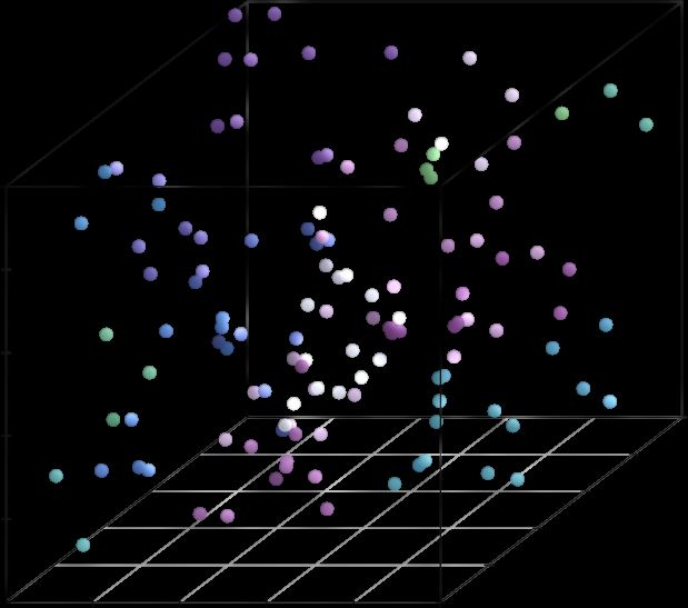
C ONTRIBUTED RESEARCH ARTICLE                                                                                           4

          (A) Delocalised transitions         (B) Localised transitions           (C) Tunneling transitions

                   Conduction band                     Conduction band                     Conduction band

              An          A
                                                      exci t ed st at e                   exci t ed st at e

               N, n, E, s, T                          B             A                     B             A
                                        Am                n, E, s, T                       n, N, E, s, T      r'

                                                                                                                   ρ'

                    Valence band                          Valence band                        Valence band

          Figure 2: Energy-band model representation of the models implemented in RLumCarlo. Letters
          represent physical model parameters and arrows indicate allowed transitions. (A) Delocalised tran-
          sition: the model consists of one single trap and one recombination centre. Transition processes
          involve the conduction band. (B) Localised transition: the model consists of two sub-conduction
          band energy levels. Charge transitions do not involve the conduction band, but take place locally
          with a constant recombination rate. (C) Tunnelling transition: The model consists of one trap and
          one recombination centre. Transitions take place from the excited state into the recombination
          centre without involving the conduction band, and the recombination rate depends on the dis-
          tance between electrons and holes. All symbols are detailed in the package manual, the package
          vignette and the main text. Side note: For the creation of the plots we used scales and ggplot2
          (https://github.com/JohannesFriedrich/EnergyBandModels).

          Implemented energy-band models

          To date, RLumCarlo ships three simple energy-band models (Figure 2) to simulate luminescence
          production using (A) delocalised transitions, (B) localised transitions, and (C) excited state tunnelling
          transitions. The models are distinguished by the allowed routes of electrons involved in the lumi-
          nescence process from one energy state to another. Only the first model (Figure 2A) involves the
          conduction band, while the models in Figures 2B and C limit the allowed electron pathways to energy
          levels below the conduction band.
               While the parameters differ from model to model and depend on the stimulation mode (heat
          or light, continuous or ramped), key entities remain alike across the models, such as the trap depth
          (the energy difference of the electron state from the conduction band) E (eV), the attempt to escape
          frequency of an electron from the trap (short: frequency factor) s (s−1 ), the temperature T (K), and
          the trapped concentration of electrons n (cm−3 ) in the trap. N (models A and B) is the total number
          of available electrons in cm−3 and ρ0 the dimensionless density of recombination centres (model C,
          Huntley, 2006). The symbols An , Am and A (model A), B and A (model B) and B, A and r 0 (model C)
          plotted next to the arrows in Figure 2 parametrise, simply put, the rates of the electronic transitions.
              The conditions of the simulations are defined through these parameters with n being the crucial
          number. Once the electrons have all recombined the simulation may still continue, but the lumi-
          nescence signal is zero. As we will detail below, the essential point of the MC simulation, from the
          physical point of view, is that these concentrations become dimensionless, absolute numbers in a finite
          system.
             Each model supports up to four different stimulation modes (Figure 3), i.e., the type of energy
          input (light or heat) and its modulation (continuous or ramped).
              As an example, we will detail the mathematical background and its implementation for delocalised
          transitions below. For all other models we may refer to the cited literature as well as the package
          manual.

          Conceptional overview of the implementation

          The basic implementation of the MC processes as software algorithm consists of two nested loops.
          The outer loop iterates over a time 0 < t 6 tmax with t ∈ R > 0. The inner part loops over particles
          0 < j 6 n with n ∈ Z. The model tests a random number, newly sampled with replacement in each
          run, against a threshold P. If the sampled random number is smaller than P, the absolute number

          The R Journal Vol. XX/YY, AAAA 20ZZ                                                       ISSN 2073-4859
C ONTRIBUTED RESEARCH ARTICLE 5
Energy input
Heat Light
ISO-TL CW-OSL/IRSL
Thermal energy (heat)
Optical energy (light)
Continuous
Modulation
Time Time
TL LM-OSL
Thermal energy (heat)
Optical energy (light)
Ramped
Time Time
Figure 3: Stimulation modes in RLumCarlo applicable to the models. ISO-TL: isothermal TL, i.e.
constant stimulation temperature over time. TL: thermal luminescence, i.e. temperature ramps (ap-
proximately linearly) over time. CW-OSL/IRSL: continuous wave optically stimulated luminescence
respectively infrared stimulated luminescence, constant optical stimulation over time. LM-OSL: lin-
early modulated optically stimulated luminescence, i.e. linearly ramped optical stimulation over
time.
of particles is reduced by one. The code below shows the basic algorithm outlined above for the
radioactive decay, which we have chosen because it can be found in standard textbooks (e.g., Landau
and Binder, 2015). Below we used R code for illustrative reasons, while the package implementation is
written in C++.
nC ONTRIBUTED RESEARCH ARTICLE 6
The OTOR model for TL can be expressed with the following set of differential equations:
dn E
= −ns exp( − ) + nc ( N − n) An (1)
dt kB T
dnc dn
=− − nc mAm (2)
dt dt
dm
ITL (t) = − = nc mAm . (3)
dt
Beyond already mentioned symbols, we used in the equations ITL , the time-dependent intensity,
and nc (cm−3 ), the current concentration of electrons in the conduction band. The concentration
of recombination centres is represented by m (cm−3 ), where for reasons of charge neutrality m =
n + nc . An and Am (both in cm3 s−1 ) are the capture coefficients for traps and recombinations centres,
respectively. k B (eV K−1 ) is the Boltzmann constant and T (K) the absolute temperature.
By assuming quasi-static equilibrium conditions (Chen et al., 2011)
dnc dn dm
, ; nc
n, n ' m (4)
dt dt dt
the resulting TL intensity becomes the general one trap equation, GOT:
dn E A m n2
ITL (t) = − = s exp(− ) . (5)
dt k B T ( N − n) An + nAm
T = T0 + β × t, (6)
with T (K) and T0 (K) being temperatures, β (K s−1 ) the (heating) rate, and t (s) the simulation time.
p(t) = s exp(− k BET ) is the rate of thermal excitation, and R = AAmn is the dimensionless retrapping ratio.
The translation into a finite system with a discrete distribution of charge carriers (cf. Mandowski and
Swiatek, 1991, 1994), can be expressed through
χn, χN → n̄, N̄ (7)
and the differential equation becomes a difference equation:
1 ∆n̄ n̄2
ITL (t) = − = p(t) . (8)
β ∆t N̄R + n̄(1 − R)
χ (cm3 ) is a constant, n̄, N̄ ∈ Z and ∆t = 1 s is an appropriate time interval. R is the dimensionless
re-trapping ratio in the finite system. To simulate the luminescence process, the related Markov
process renders similar to the theory of birth-and-death processes (e.g., Novozhilov et al., 2006), where
the population (here of electrons) decreases over continuous time with the probability to observe
a transition within ∆t being P = µn̄ ∆t (here µn̄ is the “death-rate” in s−1 ), until the population is
depleted. The so-called ‘brute force’ approach (e.g., Landau and Binder, 2015) tests sequentially the
population of electrons (n̄) per integer time step, by comparing it against a random number sampled
with replacement from a continuous distribution r ∼ U (0, 1) against the conditional probability P for
an electron to get evicted from the trap. In our case, P is calculated as follows:
n
p(t) × δt × . (9)
N̄R + n̄(1 − R)
The factor δt allows values of ∆t 6= 1 while ensuring that P
1. p(t) depends on the stimulation
mode and the chosen model. For TL (functions named run_MC_TL_()) and isothermal TL
(functions named run_MC_ISO_()) applying the localised or delocalised model p(t) becomes
E
p(t) = s exp(− ), (10)
kB T
and for TL, from tunnelling transitions it reads
E
p(t) = s exp(− ) exp(−ρ0−1/3 r 0 ), (11)
kB T
with ρ0 being the dimensionless concentration of recombination centres and r 0 the dimensionless
tunnelling radius (Huntley, 2006). The basic structure in RLumCarlo is, however, identical except
The R Journal Vol. XX/YY, AAAA 20ZZ ISSN 2073-4859C ONTRIBUTED RESEARCH ARTICLE 7
for the models based on excited state tunnelling. Here an additional outer loop iterates over the
dimensionless tunnelling radius 0 6 r 0 6 2 (Huntley, 2006).
The package design
Modelling core Modelling functions Graphical feedback
run_MC_TL_DELOC()
run_MC_TL_LOC()
run_MC_TL_TUN()
pp
Rc .
.
&
C++
.
run_MC_ISO_TUN()
Helper functions
Terminal output
plot_RLumCarlo()
summary(), c() > summary(results)
... Min.
time
:200
1st Qu.:275
Min.
mean
: 0.00000
1st Qu.: 0.06356
...
...
Min.
var
:0.0000000
1st Qu.:0.0000016
Median :350 Median : 0.91324 ... Median :0.0011150
Mean :350 Mean : 4.02468 ... Mean :0.1690922
3rd Qu.:425 3rd Qu.: 6.66946 ... 3rd Qu.:0.1059095
Internal helpers Max. :500 Max. :17.37302 ... Max. :1.5895814
Figure 4: The conceptional design of RLumCarlo. User interaction is realised via exported R functions,
one function for each model and stimulation type. For the MC runs we use C++ functions interfaced
via Rcpp. Helper functions support graphical and terminal feedback.
In Figure 4, we outline the basic layout of RLumCarlo. Two design decisions stand out: (1) Each
stimulation mode/energy-band model combination has its own exported R function commencing with
the prefix run_MC. (2) These functions interface one C++ function, each via Rcpp (Eddelbuettel et al.,
2020) (for an overview see the vignette of RLumCarlo). The R functions provide a convenient user
interface, and the C++ functions constitute the workhorse, as shown in the modelling core (Figure 4).
While the apparent reason for using C++ was speed, the implementation could have been programmed
more concisely, i.e., completely in C++ instead of interfacing C++ with R. However, we wanted to
allow code inspection by non-specialists from our field, who may wish to implement other models
alike. We found that the separation of the user interface (in R) from the modelling core (in C++) aligns
best with our premise of simplicity and flexibility.
As indicated above in the example implementation algorithm, each simulation run (Kulkarni, 1994,
used the term ‘particle tracking’) starts with n > 1 and ends at tmax , while I (t) = 0 for n = 0. In reality,
one has to execute several simulation runs separately (henceforth ‘MC clusters’, to be distinguished
from defect clusters), either to reduce the statistical fluctuation or to estimate the stochastic error
(Kulkarni, 1994). RLumCarlo runs the simulations in virtual MC clusters on single or multicore
systems using parallel (R Core Team, 2020), doParallel (Microsoft Corporation and Weston, 2020) and
foreach (Microsoft and Weston, 2020) supported by helper functions (Figure 4), to summarise results
and to provide S3-class based graphical output.
Simple illustrative examples
Simulations start with a call of the respective function, e.g., for TL using the DELOC model run_MC_TL_DELOC()
or run_MC_TL_LOC() for the LOC model, respectively (see Figures 2A-B).
resultsC ONTRIBUTED RESEARCH ARTICLE 8
(A) Delocalised transition (B) Localised transition (C) Tunnelling transition
3.5
mean mean mean
range range range
2.5
3.0
15
2.5
2.0
Signal [a.u.]
Signal [a.u.]
Signal [a.u.]
2.0
10
1.5
1.5
1.0
1.0
5
0.5
0.5
0.0
0.0
0
100 150 200 250 300 350 400 450 100 150 200 250 300 350 400 450 100 150 200 250 300 350 400 450
Temperature [°C] Temperature [°C] Temperature [°C]
Figure 5: Exemplary comparison of TL signals simulated for all three RLumCarlo models: (A)
delocalised (DELOC), (B) localised (LOC), and (C) tunnelling (TUN). General physical parameters,
such as E (1.45 eV), s (3.5 × 10¹² s−1 ) and the stimulation temperature (100–450 ◦ C) were kept constant
for all models.
(A) TL DELOC − remaining electrons (B) TL DELOC + LOC remaining electrons (C) TL LOC + DELOC − uncertainty structure
200
200
mean mean
range range
400
150
150
300
Signal [a.u.]
Signal [a.u.]
CV [%]
100
100
200
50
50
100
0
0
0
100 150 200 250 300 350 400 450 100 150 200 250 300 350 400 450 100 150 200 250 300 350 400 450
Temperature [°C] Temperature [°C] Temperature [°C]
Figure 6: (A) Plot of the remaining electrons for the TL process using the delocalised transition model
for which we show the luminescence signal in Figure 5A. (B) Plot of remaining electrons for two
models combined in one system. (C) Stochastic uncertainty structure from (B).
of Markov chains. High numbers in clusters increase the confidence in the simulation output at the
cost of more computation time.
The output can be passed to a dedicated plot function (plot_RLumCarlo()). The function supports
a couple of standard plot arguments, such as main for the title of the plot, which are passed down to
graphics::plot.default() via ... (type ?dots in the R terminal).
plot_RLumCarlo(
object = results,
legend = TRUE,
main = "(A) Delocalised transition")
The parameter n_filled can be a vector enabling different starting conditions for each MC cluster.
Figure 5A shows the graphical output for delocalised transitions along with the simulation results for
TL stimulation using localised (Figure 5B) and tunnelling transitions (Figure 5C). The output is an
object of class RLumCarlo_Model_Output, which is a list comprising a multi-dimensional array (one
slice per MC cluster) with the resulting luminescence signal and a numeric vector for the stimulation
time.
Currently we provide S3-generics for summary() and c(). The first one is also used internally by
plot_RLumCarlo() to melt the array into a data.frame before plotting. The plot output adapts to the
used stimulation mode provided via an attribute with each output object.
A straightforward application for this kind of simulations is the study of the impact of physical
parameters on the luminescence signal output and the estimation of the stochastic uncertainties, which
cannot be achieved with the deterministic approach of differential equations.
We provide more, always up-to-date examples with the package vignette, where we also compiled
a table with meaningful physical parameter ranges for each model.
The R Journal Vol. XX/YY, AAAA 20ZZ ISSN 2073-4859C ONTRIBUTED RESEARCH ARTICLE 9
Advanced examples and further considerations
The examples so far presented may not appear very sophisticated, and still, they allow insight that
goes beyond a simple educational purpose of simulating luminescence based on phenomenological
models. Pagonis et al. (2020), who used a preliminary version of RLumCarlo, addressed in detail the
stochastic uncertainties of TL and OSL models. These uncertainties come into play in nano-dosimetric
materials with a small number of defect clusters where the “finite-size” (Mandowski and Swiatek,
1991) of the system starts to matter in terms of a presumed spatial correlation of defect cluster groups.
To some extent, this should also be true for systems exposed to high-energy radiation causing defect
clusters (e.g, Mandowski and Swiatek, 1991; Mandowski and Świaltek, 1992). Previously in this paper,
we have used the term ‘MC clusters’. For a start, in RLumCarlo, ‘MC clusters’ entail independent and
continuous Monte Carlo Markov chains employed to simulate luminescence production; starting with
a particular number of electrons in the system. Whether the processes are run in parallel or sequentially
has no impact on the outcome, except for computation speed. In other words, ‘MC clusters’ carry no
meaning regarding the underlying physics. However, as mentioned above, MC clusters from different
models (with the same stimulation mode) can be concatenated (see Figure 6B-C) to simulate defect
clusters (also, dosimetric clusters), to which we can attribute physical meaning.
Spatial correlation
To simulate a three-dimensional (dosimetric) system, we can add meaning to MC clusters by rein-
terpreting them as dosimetric clusters. From the modelling perspective, nothing changes, but MC
clusters gain a connotation of having a physical meaning.
Figure 7A illustrates the situation of model combinations transferred into a virtual, three-dimen-
sional dosimetric system. Since all defect clusters are distributed evenly over the system, the distance
to each neighbouring point is identical, and it is a constant rather than a variable. In other words, the
spatial distance between neighbouring points does not matter and is of no relevance for the simulation
but here chosen for illustrative reasons only. Figure 7B represents a situation that takes one step
further. Here the points are randomly distributed over the system and points form groups (defect
cluster groups). Additionally, RLumCarlo supports mixing of models for the same stimulation mode
as in Figure 7A (not shown here). The driving idea of the implementation is the assumption of an
individual spatial ordering of defects in a, e.g., quartz crystal to which the luminescence production
process might be assigned based on models mentioned above.
Such a system can be created in RLumCarlo via create_ClusterSystem(). The function distributes
points randomly with their coordinates
x1 , y1 , z1 , ..., xk , yk , zk ∼ U (0, 1) | k ∈ Z. (12)
A B C
Model 1 Model 1
Model 2
transfer function
Model 3 enabling charge
exchange based
on their spatial
distance e-
e-
e-
Model 2 e-
Cluster e-
e-
groups
Model 3
Cluster
groups
Mixing of models, Mixing of models, Mixing of models,
no spatial correlation, no interaction simple spatial correlation, no interaction advanced spatial correlation, interaction
Figure 7: A dosimetric system with three possible approaches of cluster correlation and interaction.
(A) Models can be mixed but no spatial correlation is realised and no interaction possible. This is
the basic mode in RLumCarlo. (B) Clusters are grouped by their Euclidean distance and models can
be mixed. Electrons are distributed according to the spatial distance of clusters and also models can
be mixed (not shown in the figure). The advanced mode in RLumCarlo. (C) Clusters can interact
with each other and even exchange electrons. This last stage is subject to future developments of
RLumCarlo.
Then the Euclidean distance between the points is determined with stats:dist(), which is
used by stats:hclust() to group the defect clusters (Ξ). To avoid too many small groups, we then
cut the cluster tree using stats:cutree(), with the outcome shown in Figure 7B. The selection of
stats:hclust() and stats:cutree() for defining the clusters is somewhat arbitrary and might be
The R Journal Vol. XX/YY, AAAA 20ZZ ISSN 2073-4859C ONTRIBUTED RESEARCH ARTICLE 10
refined in the future. Therefore, more research, supported by measurements, is needed.
Now, any function from RLumCarlo can be used and the output of create_ClusterSystem() is
taken as input for the argument clusters. For example:
run_MC_TL_LOC(s = 3.5e12, E = 1.45, n_filled = 1000,
clusters = create_ClusterSystem(100))
creates a system with 100 randomly distributed defect clusters. If the simulation is run in such
a mode, the meaning of n_filled changes. Previously it defined the number of electrons in each
cluster (n̄cli ), however, now the same parameter defines the total number of electrons in the entire
system. The number of electrons in the ith cluster (n̄cli ) is then an integer fraction of electrons available
in each cluster group (n̄Ξi = n_filled/NΞ , with NΞ the total number of cluster groups). The more
clusters are in one group, the less electrons are available per cluster in the group and vice versa. While
this is a very simple approach, it allows us to simulate basic spatial correlation. Figure 7C drafts a
better way of mimicking spatial interaction of clusters, which is, however, not yet part of RLumCarlo.
While it would be, based on the designed system, easy from the programming perspective, the needed
equations to describe to exchange electrons are yet to be developed.
Comparison to RLumModel
In the remainder, we want to compare simulation results from RLumCarlo with other types of so-
lutions, such as RLumModel which uses coupled differential equations to simulate luminescence
production. RLumModel was selected since it was developed by some of the authors of this contribu-
tion, however, in theory, simple scripts using any existing model to simulate luminescence should
work as well (as long as the models are comparable).
In contrast to RLumCarlo, RLumModel input values for physical parameters are preset. RLum-
Model encourages users to write a virtual luminescence signal measurement sequence, which is
processed based on a pre-defined model with preset physical parameters.
For the comparison, we have selected a TL curve simulated with the luminescence model for
quartz by Bailey (2001).
outputC ONTRIBUTED RESEARCH ARTICLE 11
RLumModel vs RLumCarlo
Bailey 2001
1.0
RLumModel
RLumCarlo
0.8
0.6
Norm. TL
0.4
0.2
0.0
100 200 300 400
Temperature [°C]
Figure 8: Simulation results of RLumModel and RLumCarlo. Qualitatively both approaches show a
good match.
et al. (2018). In summary, the results in Figure 8 show that even complex luminescence models can be
simulated through the combination of clusters, which brings us back to the initial ‘simplicity’ premise
of RLumCarlo. Still, a big ‘but’ remains. Luminescence models such as those proposed by Bailey
(2001) or Pagonis et al. (2008) go beyond single curve simulations. Their purpose is to deliver a general
kinetic model for luminescence production of, e.g., quartz including the simulation of trap filling by
irradiation and the simulation of the thermal activation history of the mineral. By contrast, so far all
simulations in RLumCarlo start with a predefined number of electrons in a trap and are not by default
limited to a specific dosimeter. RLumCarlo can model more complex luminescence phenomena,
but not in a pre-described way out of the box. Instead, RLumCarlo is more like a patch box with
each model representing a socket ready to be flexibly rewired in many ways to simulate cascades of
luminescence production. Due to the nature of the chosen MC approach, in theory (adhering to the
patch box picture) the number of sockets is not limited.
Summary
The modelling of luminescence phenomena (cold light) of semiconductors and insulators after having
received ionising radiation is a challenging task. MC methods allow setting up flexible and simple
systems to simulate luminescence with a finite number of charge carriers. This enables users to address
effects usually observed for nano-dosimetric systems, and it provides insight into the stochastic
uncertainty structure. We presented RLumCarlo, which renders, to our best knowledge, the first
open-source and ready-to-use compilation of basic MC luminescence models for different stimulation
modes (so far CW-OSL, LM-OSL, ISO-TL and TL). We showed that the output from different models,
which are simulated in separate MC chains in virtual clusters, can be combined to either simulate
more complex systems or to mimic simple spatial correlations between cluster groups. The way of
the implementation does not limit RLumCarlo to a specific dosimeter (e.g., quartz). In this light,
RLumCarlo can be used in education, but also in research to test the impact of model parameters,
such as cluster sizes and related stochastic uncertainties. Furthermore, RLumCarlo can help in in
formulating research hypotheses and test them with commonly accepted or new models, still to be
developed.
Future work will implement more models to run as MC simulation, e.g., for irradiation processes
in crystals (including its luminescence output: radiofluorescence) and for an advanced interaction of
clusters.
Acknowledgements
We thank two anonymous reviewers for their thorough reviews and constructive suggestions, which
helped to improve our manuscript. Furthermore, we are grateful to the CRAN team in general for
their tireless efforts of keeping such a great resource alive and in particular for their patience during
the initial submission of RLumCarlo. Alex Roy Duncan is thanked for his support on the package
development during our stay in Westminster. The development of RLumCarlo benefited from the
support of various funding bodies. The initial work by JF, SK and CS was supported by the Deutsche
Forschungsgemeinschaft (2015–2018, DFG SCHM 3051/4-1, “Modelling quartz luminescence signal
dynamics relevant for dating and dosimetry”). Later financial support was secured through the project
The R Journal Vol. XX/YY, AAAA 20ZZ ISSN 2073-4859C ONTRIBUTED RESEARCH ARTICLE 12
“ULTIMO: Unifying Luminescence Models of quartz and feldspar” granted by the Deutscher Akademischer
Austauschdienst (DAAD PPP USA 2018, ID: 57387041). SK was supported by the LabEx LaScArBx
(ANR - n.◦ ANR-10-LABX-52) until 2019. From 2020, SK has received funding from the European
Union’s Horizon 2020 research and innovation programme under the Marie Skłodowska-Curie grant
agreement No 844457 (CREDit). This is IPGP contribution number 4202.
Bibliography
M. J. Aitken. Thermoluminescence dating. Studies in archaeological science. Academic Press, 1985. [p]
M. J. Aitken. An Introduction to Optical Dating. Oxford University Press, 1998. [p]
R. M. Bailey. Towards a general kinetic model for optically and thermally stimulated luminescence of
quartz. Radiation Measurements, 33(1):17–45, 2001. URL https://doi.org/10.1016/S1350-4487(00)
00100-1. [p]
M. D. Bateman. Handbook of Luminescence Dating. Whittles Publishing, 2019. [p]
L. Bøtter-Jensen, S. W. S. McKeever, and A. G. Wintle. Optically Stimulated Luminescence Dosimetry.
Elsevier Science B.V., 2003. [p]
C. Burow, S. Kreutzer, M. Dietze, M. C. Fuchs, M. Fischer, C. Schmidt, and H. Brückner. RLumShiny
- A graphical user interface for the R Package ’Luminescence’. Ancient TL, 34:22–32, 2016. URL
http://ancienttl.org/ATL_34-2_2016/ATL_34-2_Burow_p22-32.pdf. [p]
C. Burow, U. T. Wolpert, and S. Kreutzer. RLumShiny: ’Shiny’ Applications for the R Package ’Luminescence’,
2019. URL https://CRAN.R-project.org/package=RLumShiny. R package version 0.2.2. [p]
R. Chen and S. W. S. McKeever. Theory of Thermoluminescence and Related Phenomena. WORLD
SCIENTIFIC, 1997. [p]
R. Chen, J. L. Lawless, and V. Pagonis. A model for explaining the concentration quenching of
thermoluminescence. Radiation Measurements, 46:1380–1384, 2011. URL https://doi.org/10.1016/
j.radmeas.2011.01.022. [p]
C. Christophe, A. Philippe, S. Kreutzer, and G. Guerin. BayLum: Chronological Bayesian Models Inte-
grating Optically Stimulated Luminescence and Radiocarbon Age Dating, 2018. URL https://CRAN.R-
project.org/package=BayLum. R package version 0.1.3. [p]
F. Daniels, C. A. Boyd, and D. F. Saunders. Thermoluminescence as a Research Tool. Science, 117(3040):
343–349, 1953. URL https://doi.org/10.1126/science.117.3040.343. [p]
D. Eddelbuettel, R. Francois, J. Allaire, K. Ushey, Q. Kou, N. Russell, D. Bates, and J. Chambers. Rcpp:
Seamless R and C++ Integration, 2020. URL https://CRAN.R-project.org/package=Rcpp. R package
version 1.0.5. [p]
J. Friedrich, S. Kreutzer, and C. Schmidt. Solving ordinary differential equations to understand
luminescence: ’RLumModel’ an advanced research tool for simulating luminescence in quartz using
R. Quaternary Geochronology, 35(C):88–100, 2016. URL https://doi.org/10.1016/j.quageo.2016.
05.004. [p]
J. Friedrich, S. Kreutzer, and C. Schmidt. Radiofluorescence as a detection tool for quartz luminescence
quenching processes. Radiation Measurements, 120:33–40, 2018. URL https://doi.org/10.1016/j.
radmeas.2018.03.008. [p]
J. Friedrich, S. Kreutzer, and C. Schmidt. RLumModel: Solving Ordinary Differential Equations to
Understand Luminescence, 2020. URL https://CRAN.R-project.org/package=RLumModel. R package
version 0.2.7. [p]
N. Grögler, F. G. Houtermans, and H. Stauffer. Radiation damage as a research tool for geology and
prehistory. In 5° Rassegna Internazionale Elettronica E Nucleare, Supplemento Agli Atti Del Congresso
Scientifico, pages 5–15. Sezione Nucleare, 1958. [p]
A. Halperin and A. A. Braner. Evaluation of Thermal Activation Energies from Glow Curves. Physical
Review, 117(2):408–415, 1960. URL https://doi.org/10.1103/PhysRev.117.408. [p]
Y. S. Horowitz, I. Eliyahu, and L. Oster. Kinetic Simulations of Thermoluminescence Dose Response:
Long Overdue Confrontation with the Effects of Ionisation Density. Radiation Protection Dosimetry,
172(4):524–540, 2017. URL https://doi.org/10.1093/rpd/ncv495. [p]
The R Journal Vol. XX/YY, AAAA 20ZZ ISSN 2073-4859C ONTRIBUTED RESEARCH ARTICLE 13
F. G. Houtermans and H. Stauffer. Thermolumineszenz als Mittel zur Untersuchung der Temperatur -
und Strahlungsgeschichte von Mineralien und Gesteinen. Helvetica Physica Acta, 30:274–277, 1957.
[p]
D. J. Huntley. An explanation of the power-law decay of luminescence. Journal of Physics: Condensed
Matter, 18(4):1359–1365, 2006. URL https://doi.org/10.1088/0953-8984/18/4/020. [p]
R. P. Johnson. Luminescence of Sulphide and Silicate Phosphors. Journal of the Optical Society of America,
29(9):387–391, 1939. URL https://doi.org/10.1364/JOSA.29.000387. [p]
S. Kreutzer, C. Schmidt, M. C. Fuchs, M. Dietze, M. Fischer, and M. Fuchs. Introducing an R package
for luminescence dating analysis. Ancient TL, 30(1):1–8, 2012. URL http://ancienttl.org/ATL_30-
1_2012/ATL_30-1_Kreutzer_p1-8.pdf. [p]
S. Kreutzer, C. Burow, M. Dietze, M. C. Fuchs, C. Schmidt, M. Fischer, J. Friedrich, S. Riedesel,
M. Autzen, and D. Mittelstrass. Luminescence: Comprehensive Luminescence Dating Data Analysis,
2020. URL https://CRAN.R-project.org/package=Luminescence. R package version 0.9.8. [p]
R. N. Kulkarni. The Development of the Monte Carlo Method for the Calculation of the Thermolumi-
nescence Intensity and the Thermally Stimulated Conductivity. Radiation Protection Dosimetry, 51(2):
95–105, 1994. URL https://doi.org/10.1093/oxfordjournals.rpd.a082126. [p]
D. P. Landau and K. Binder. A Guide to Monte Carlo Simulations in Statistical Physics. Cambridge
University Press, 2015. [p]
K. Mahesh, P. S. Weng, and C. Furetta. Thermoluminescence in solids and its application. Thermolumines-
cence in solids and its application. Nuclear Technology Publishing, England, 1989. [p]
A. Mandowski and J. Świaltek. Monte Carlo simulation of thermally stimulated relaxation kinetics
of carrier trapping in microcrystalline and two-dimensional solids. Philosophical Magazine B, 65(4):
729–732, 1992. URL https://doi.org/10.1080/13642819208204910. [p]
A. Mandowski and J. Swiatek. On the determination of trap parameters from TSC spectra in finite-
size systems. In 7th International Symposium on Electrets (ISE 7), pages 588–593. IEEE, 1991. URL
https://doi.org/10.1109/ISE.1991.167278. [p]
A. Mandowski and J. Swiatek. Monte Carlo simulation of TSC and TL in spatially correlated systems.
In 8th International Symposium on Electrets (ISE 8), pages 461–466. IEEE, 1994. URL https://doi.
org/10.1109/ISE.1994.514813. [p]
S. W. S. McKeever. Thermoluminescence of solids. Thermoluminescence of solids. Cambrigde University
Press, 1983. [p]
Microsoft and S. Weston. foreach: Provides Foreach Looping Construct, 2020. URL https://CRAN.R-
project.org/package=foreach. R package version 1.5.1. [p]
Microsoft Corporation and S. Weston. doParallel: Foreach Parallel Adaptor for the ’parallel’ Package, 2020.
URL https://CRAN.R-project.org/package=doParallel. R package version 1.0.16. [p]
E. Newton Harvey. A history of luminescence from the earliest times until 1900. Philadelphia, American
Philosophical Society, 1957. [p]
A. S. Novozhilov, G. P. Karev, and E. V. Koonin. Biological applications of the theory of birth-and-death
processes. Briefings in Bioinformatics, 7(1):70–85, 2006. URL https://doi.org/10.1093/bib/bbk006.
[p]
V. Pagonis and R. Chen. Monte Carlo simulations of TL and OSL in nanodosimetric materials and
feldspars. Radiation Measurements, 81:262–269, 2015. URL https://doi.org/10.1016/j.radmeas.
2014.12.009. [p]
V. Pagonis, G. Kitis, and C. Furetta. Numerical and Practical Exercises in Thermoluminescence. Springer,
2006. [p]
V. Pagonis, E. Balsamo, C. Barnold, K. Duling, and S. McCole. Simulations of the predose technique
for retrospective dosimetry and authenticity testing. Radiation Measurements, 43(8):1343–1353, 2008.
URL https://doi.org/10.1016/j.radmeas.2008.04.095. [p]
V. Pagonis, E. Gochnour, M. Hennessey, and C. Knower. Monte Carlo simulations of luminescence
processes under quasi-equilibrium (QE) conditions. Radiation Measurements, 67(C):67–76, 2014. URL
https://doi.org/10.1016/j.radmeas.2014.06.005. [p]
The R Journal Vol. XX/YY, AAAA 20ZZ ISSN 2073-4859C ONTRIBUTED RESEARCH ARTICLE 14
V. Pagonis, J. Friedrich, M. Discher, A. Müller-Kirschbaum, V. Schlosser, S. Kreutzer, R. Chen, and
C. Schmidt. Excited state luminescence signals from a random distribution of defects - A new
Monte Carlo simulation approach for feldspar. Journal of Luminescence, 207:266–272, 2019. URL
https://doi.org/10.1016/j.jlumin.2018.11.024. [p]
V. Pagonis, S. Kreutzer, A. R. Duncan, E. Rajovic, C. Laag, and C. Schmidt. On the stochastic uncertain-
ties of thermally and optically stimulated luminescence signals: A Monte Carlo approach. Journal of
Luminescence, 219:116945, 2020. URL https://doi.org/10.1016/j.jlumin.2019.116945. [p]
J. Peng. tgcd: Thermoluminescence Glow Curve Deconvolution, 2020. URL https://CRAN.R-project.org/
package=tgcd. R package version 2.5. [p]
J. Peng and B. Li. numOSL: Numeric Routines for Optically Stimulated Luminescence Dating, 2018. URL
https://CRAN.R-project.org/package=numOSL. R package version 2.6. [p]
J. Peng and V. Pagonis. Simulating comprehensive kinetic models for quartz luminescence using the R
program KMS. Radiation Measurements, 86:63–70, 2016. URL https://doi.org/10.1016/j.radmeas.
2016.01.022. [p]
J. Peng, Z. Dong, F. Han, H. Long, and X. Liu. R package numOSL: numeric routines for optically
stimulated luminescence dating. Ancient TL, 31(2):41–48, 2013. URL http://ancienttl.org/ATL_31-
2_2013/ATL_31-2_Peng_p41-48.pdf. [p]
J. Peng, Z. Dong, and F. Han. tgcd: An R package for analyzing thermoluminescence glow curves.
SoftwareX, pages 1–9, 2016. URL https://doi.org/10.1016/j.softx.2016.06.001. [p]
A. Philippe, G. Guérin, and S. Kreutzer. BayLum - An R package for Bayesian analysis of OSL ages: An
introduction. Quaternary Geochronology, 49:16–24, 2019. URL https://doi.org/10.1016/j.quageo.
2018.05.009. [p]
R Core Team. R: A Language and Environment for Statistical Computing. R Foundation for Statistical
Computing, Vienna, Austria, 2020. URL https://www.R-project.org/. [p]
J. T. Randall and M. H. F. Wilkins. Phosphorescence and Electron Traps. I. The Study of Trap Distribu-
tions. Proceedings of the Royal Society of London A: Mathematical, Physical and Engineering Sciences, 184
(999):365–389, 1945. URL https://doi.org/10.1098/rspa.1945.0024. [p]
F. Urbach. Zur Lumineszenz der Alkalihalogenide II. Messungsmethoden; erste Ergebnisse; zur Theo-
rie der Thermolumineszenz. Sitzungsberichte der Akademie der Wissenschaften in Wien, Mathematisch-
Naturwissenschaftliche Klasse, Abt. IIa, Mathematik, Astronomie, Physik, Meteorologie und Technik, 139:
363–372, 1930. [p]
A. G. Wintle. Thermal Quenching of Thermoluminescence in Quartz. Geophysical Journal of the
Royal Astronomical Society, 41:107–113, 1975. URL https://doi.org/10.1111/j.1365-246X.1975.
tb05487.x. [p]
E. G. Yukihara and S. W. S. McKeever. Optically Stimulated Luminescence. Wiley, 2011. [p]
Sebastian Kreutzer
Geography & Earth Sciences, Aberystwyth University
Aberystwyth
SY23 3DB, Wales, United Kingdom
IRAMAT-CRP2A, UMR 5060, CNRS-Université Bordeaux Montaigne
Maison de l’Archéologie
Esplanade des Antilles
36607 Pessac Cedex, France
ORCiD: 0000-0001-9166-4563
sebastian.kreutzer@aber.ac.uk
Johannes Friedrich
Chair of Geomorphology, University of Bayreuth
Universitätsstr. 30
95447 Bayreuth, Germany
ORCiD: 0000-0002-0805-9547
johannes.friedrich@posteo.de
The R Journal Vol. XX/YY, AAAA 20ZZ ISSN 2073-4859C ONTRIBUTED RESEARCH ARTICLE 15
Vasilis Pagonis
Physics Department, McDaniel College
Westminster, MD 21157, USA
ORCiD: 0000-0002-4852-9312
vpagonis@mcdaniel.edu
Christian Laag
Université de Paris, Institut de Physique du Globe de Paris, CNRS
75005 Paris, France
Chair of Geomorphology, University of Bayreuth
95447 Bayreuth, Germany
ORCiD: 0000-0002-6012-1029
laag@ipgp.fr
Ena Rajovic
Chair of Geomorphology, University of Bayreuth
95447 Bayreuth, Germany
ena.rajovic@uni-bayreuth.de
Christoph Schmidt
Institute of Earth Surface Dynamics, University of Lausanne
1015 Lausanne, Switzerland
ORCiD: 0000-0002-2309-3209
christoph.schmidt@unil.ch
The R Journal Vol. XX/YY, AAAA 20ZZ ISSN 2073-4859You can also read