Predictability of extreme meteo-oceanographic events in the Adriatic Sea
←
→
Page content transcription
If your browser does not render page correctly, please read the page content below
Quarterly Journal of the Royal Meteorological Society                      Q. J. R. Meteorol. Soc. 136: 400–413, January 2010 Part B

          Predictability of extreme meteo-oceanographic events
                             in the Adriatic Sea
L. Cavaleri,a * L. Bertotti,a R. Buizza,b A. Buzzi,c V. Masato,a G. Umgiessera and M. Zampieric
                                                     a
                                                ISMAR-CNR, Venice, Italy
                                                 b ECMWF,
                                                        Reading, Berkshire, UK
                                               c ISAC-CNR, Bologna, Italy

                     *Correspondence to: L. Cavaleri, ISMAR-CNR, Castello 1364, 30122 Venice, Italy.
                                            E-mail: luigi.cavaleri@ismar.cnr.it

             The performance of state-of-the-art meteorological and oceanographic numerical
             systems in predicting the sea state in the Adriatic Sea during intense storms is
             assessed. Two major storms that affected Venice are discussed. The first storm
             occurred on 4 November 1966, when Venice suffered its most dramatic flood
             event. The damage and loss of life caused by the storm and the associated flood
             were extremely high also because the event was poorly forecast. The 1966 event
             is reanalysed using state-of-the-art meteorological and oceanographic numerical
             systems to investigate whether the poor forecast quality was due to a lack of data
             or of suitable numerical modelling. The second severe storm took place on 22
             December 1979, when Venice experienced the second-worst ‘acqua-alta’ conditions
             in recorded history. Results show that with the present numerical systems both
             storms and associated wave and surge conditions could have been forecast several
             days in advance. Potential implications for the prediction of more frequent less
             intense storms are discussed, and a suitably enhanced system based on a global
             meteorological model and a limited area one is outlined. Copyright c 2010 Royal
             Meteorological Society

             Key Words:    wind waves; surge; historical storms; meteorological modelling; downscaling

             Received 22 October 2008; Revised 1 October 2009; Accepted 27 November 2009; Published online in Wiley
             InterScience 1 February 2010

             Citation: Cavaleri L, Bertotti L, Buizza R, Buzzi A, Masato V, Umgiesser G, Zampieri M. 2010. Predictability
             of extreme meteo-oceanographic events in the Adriatic Sea. Q. J. R. Meteorol. Soc. 136: 400–413.
             DOI:10.1002/qj.567

1.   Introduction: The historical storms                            afterwards. The interested reader is referred to, among
                                                                    others, Fea et al. (1968), Warner and Hsu (2000), Bertò
On 4 November 1966 an exceptional storm hit the                     et al. (2005), De Zolt et al. (2006) and Malguzzi et al. (2006).
central and north-eastern part of Italy with very intense              Most of the past studies have focused on the
precipitation over large areas and strong winds over the            meteorological and hydrological components of this storm,
Adriatic Sea, east of the Italian peninsula (see Figure 1 for an    often dealing specifically with the estimate and distribution
analysis of that time of the weather situation at the surface).     of the amount of rain and the consequent flood of Florence
The storm caused the flood of two of the greatest historical        by the Arno River and with the widespread floods and
towns of Italy, Florence and Venice, inflicted severe damage        landslides in the eastern Alps (see, for example, the recent
to the economic and artistic patrimony of these and other           paper by Malguzzi et al. (2006)). In the present paper we
towns and villages in central and north-eastern Italy, and          focus on the oceanographic aspect of the storm, hence on
claimed the lives of more than 100 people. Because of this,         the flood of Venice due to the exceptional surge of the
and since at that time the quality of a weather forecast            Adriatic Sea. More specifically, our aim is to analyse the
was very limited, the storm has been extensively studied            predictability not only of the atmospheric, but also of the
         Copyright
                   c 2010 Royal Meteorological Society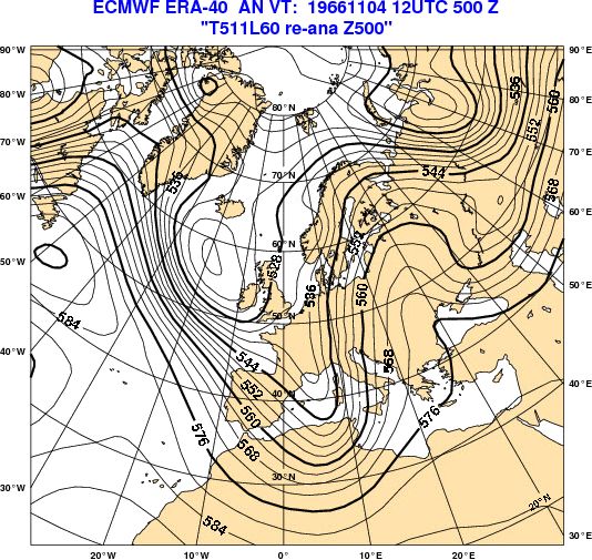
Predictability of Extreme Events in the Adriatic 401
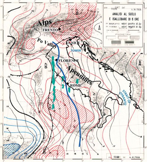
Figure 1. Weather map re-elaborated from hand-drawn analysis published in Fea et al. (1968). The basic meteorological fields refer to 4 November 1966,
0000 UTC. Continuous black lines: mean-sea-level pressure −1000 hPa (contour interval 2 hPa). Coloured thin lines: pressure tendency in 6 hours (blue:
positive; red: negative; contour interval hPa/6h). Wind barbs in knots. Low pressure centres: B; high pressure: A. The green spots reproduce reflectivity
maxima of the meteorological radar in Rome Fiumicino at 0040 UTC, same day. The thick line indicates the position of the cold front at 1200 UTC of the
same day (after Malguzzi et al., 2006). The highlighted coastline borders the Adriatic Sea. The red circle shows the position of the oceanographic tower
(see Figure 5), 15 km off the coast of Venice.
marine conditions on the Adriatic Sea associated with this 13 years later, on 22 December 1979. Although this storm
storm. As mentioned above, at the time of the storm there did not reach the severity level of the 1966 one, it led to
was practically no anticipation of what was about to come. the second-ranked record sea level in Venice. Although we
At that time there was no operational numerical modelling recognize that it is difficult to generalize conclusions drawn
guide available to the forecasters, so forecasts were based from the analysis of two storms, we think that this study
essentially on the synoptic interpretation of the available can give some useful indications of general validity, and can
charts, guided by personal training and experience. In the guide the development of future alert systems.
case of the 1966 storm, unfortunately, this experience was We begin our paper with a description, in section 2, of
not enough to help forecasters to issue a skilful forecast a the key morphological characteristics of the area affected
few days before the storm, mainly because of the exceptional by the event, and, in section 3, of the atmospheric and sea
nature, and rarity, of the event. conditions during the two storms. In section 4 we present
One of the questions that we will be addressing is whether in detail the methodology we have followed and the data
the atmospheric data available prior to the storm (which did we have used. The two following sections, 5 and 6, are
not include all the satellite data that are presently available, devoted to the presentation of the results of the numerical
which nowadays constitute more than 90% of the data used simulations of the two storms. We discuss our findings and
to estimate the current state of the atmosphere) would have draw our conclusions in the final section 7.
been sufficient to issue an alert if the analysis and modelling
tools of today had been available. Could these two events be 2. Morphological and physical characteristics of the area
predicted a few days in advance? More precisely, how long of interest
in advance could the sea conditions have been predicted?
This is explored using two sources of meteorological data: The Adriatic Sea (Figure 1) is an elongated basin to the
a global model and a limited area one, both using the same east of Italy, enclosed between the Italian peninsula and the
background data. This will allow, if not firm conclusions, Balkans. It is about 750 km long, 200 km wide, aligned in
some discussion on the possible advantages of the two the north-west to south-east direction. At its southern end
approaches. it is connected with the Mediterranean Sea via the narrow
The same methodology has been applied to a second, still Strait of Otranto. The sea is shallow in its northern part, the
exceptional, storm that affected the western Mediterranean bottom sloping down from the northern coast at a gradient
Copyright
c 2010 Royal Meteorological Society Q. J. R. Meteorol. Soc. 136: 400–413 (2010)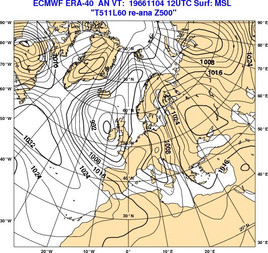
402                                                               L. Cavaleri et al.

(a)                                                                          (b)

Figure 2. ERA-40 maps of (left) geopotential heights at 500 hPa (contour interval 40 m) and (right) of mean-sea-level pressure (contour interval 4 hPa)
at 1200 UTC 4 November 1966. This figure is available in colour online at www.interscience.wiley.com/journal/qj

of 1 in 1000. Beyond the 200-metre isobath the bottom                        3.     The two flood events in Venice of 1966 and 1979
deepens suddenly, remaining so until Otranto except for the
narrow strip of shallow water along the Italian peninsula.                   3.1.    The flood of 4 November 1966
   The bordering orography affects the local wind patterns
substantially. The whole eastern border is characterised                     Between 1 and 2 November, a deep tropospheric trough
by the long ridge of the Dinaric Alps. Along the Italian                     positioned over Spain started intensifying and rotating
coast the sea is bordered by the Apennines mountain range                    anticlockwise. By 3 November, the trough deepened very
for most of its length. This orographic configuration has                    rapidly over Spain, and strong south-easterly and then
a strong influence on the low-level winds that affect the                    southerly winds started affecting the mid-troposphere over
Adriatic Sea, in particular on the sirocco, a south-easterly                 the Italian peninsula. At the surface on 3 November
wind often blowing along the whole length of the basin.                      cyclogenesis started over Spain. The surface cyclone moved
Sirocco conditions often cause flooding of the coastal areas                 over the western Mediterranean and was reinforced by
facing the northern parts of the Adriatic Sea, e.g. the                      a secondary, small-scale depression coming from North
Venice lagoon. This was actually the case in November                        Africa. At the same time, an anticyclone over the Balkans
1966 (Figure 1), when the flow at the surface was channelled                 intensified in place. The result was a strong southerly flow
by the bordering orography along the longitudinal axis of                    over the Adriatic (Figure 2, left panel) that at the surface
the basin. The reader is referred to Pirazzoli and Tomasin                   (right panel), channelled by the bordering orography, led to
(2003) for a more detailed description of the main types of                  a strong sirocco wind over the whole basin.
flow conditions that affect the Adriatic area.                                  As noted in Malguzzi et al. (2006), although the low-
                                                                             pressure centre located over northern Italy was not very
   For the following discussion it is important to note that,
                                                                             deep (see right panel), the west-to-east pressure gradient,
at a given position and for a given wind stress, when the
                                                                             and hence the south-easterly wind over the Adriatic Sea,
ocean is in dynamical equilibrium, then the surface spatial
                                                                             was very strong. On 4 November (Figure 1), the wind was
gradient of the sea elevation associated with a surge tends
                                                                             further intensified by the advancing cold front from the
to increase inversely to the local depth (see Pugh (1987)
                                                                             west, assuming the character of a pre-frontal low-level jet.
for an analysis of the dynamics of a surge, and Tomasin                      As will be discussed again later, the correct positioning and
(2005) for a description of its local characteristics). The sea              timing of this cold front played a crucial role in the accuracy
becomes shallower while moving northwards towards the                        of the forecasts.
Venetian coast. Therefore, when the sirocco reaches these                       No report of the surface wind speed over the sea is
most northerly positions, we expect to find here the steepest                available, but an unofficial anemometer located at the edge
gradients of the sea elevation and therefore an enhanced                     of the Venetian lagoon, very close to the sea coastline,
peak of the surge towards the coast.                                         reported sustained winds close to or above 20 m/s from
   Once the storm is over and if, as expected, the basin is                  0800 until 1600 UTC 4 November. As might be expected, no
out of balance, a sequence of oscillations (seiche) of the                   wave measurements were available, but the storm destroyed
whole basin is initiated with two dominant periods, 11 and                   the final 100–200 metres of the jetties bordering the three
22 hours, the latter being the stronger one (Tomasin, 2005).                 inlets connecting the Venice lagoon to the sea. Some of these
Their amphidromic (pivotal) points are respectively in the                   jetties housed open-sea tide gauges that were obviously
middle and at the lower end of the Adriatic Sea. The largest                 wiped out. Tide records exist from the Venice area, inside
oscillations are found in its northern part, adding to the                   the lagoon. However, based on previous experience, these
Venice tide.                                                                 tide gauges had been designed for a maximum level of
            Copyright
                      c 2010 Royal Meteorological Society                                Q. J. R. Meteorol. Soc. 136: 400–413 (2010)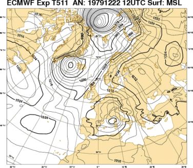
Predictability of Extreme Events in the Adriatic                                                           403

Figure 3. Time history of the flood of 4 November 1966 in Venice. Ordinate scale in m. Dashed line: meteorological tide; solid line: record; dotted line:
astronomical tide. The vertical and horizontal lines, plus the arrow, point out the time of the peak and the corresponding astronomical tide level. This
figure is available in colour online at www.interscience.wiley.com/journal/qj

1.80 m above the nominal sea level† . The maximum sea
level reached during this storm was estimated at +1.94 m
from the marks left on the walls by the oil exiting from
the flooded tanks and floating on top of the water. The
officially accepted time history of the flood is given by the
solid line in Figure 3, showing also (a full description will
be given in section 5) the astronomical tide and the isolated,
by difference, meteorological contribution. It is worthwhile
to remember that the part of the diagram above 1.80 m
was guessed and traced by hand later on. Note also that the
water in the lagoon was oscillating wildly, reaching different
levels at different times and positions. Hence also the 1.94 m
figure must be considered accurate only to within a few
centimetres.
   Compared to the statistics derived from previous data,
recorded since 1872, the 1966 event stands out dramatically,
and it was variously judged (Cecconi et al., 1999) to have
a return period of 150–300 years. It is interesting to note
that two comparable, but not properly quantified, events                      Figure 4. Synoptic situation, according to the T511 ECMWF analysis,
                                                                              over Europe at 1200 UTC 22 December 1979. Mean-sea-level pressure
reported in historical documents happened in 1822 and                         (contour interval 4 hPa). This figure is available in colour online at
1867, when no instrumental measurements were taken                            www.interscience.wiley.com/journal/qj
(Camuffo, 1993). It seems likely that the latter event triggered
the start of official measurements.
   Another remarkable detail that highlights even further                     was 23 cm higher than the nominal value, established back
the exceptional character of the 1966 storm is that the flood                 in 1896 and still in use today.
was entirely due to the storm surge, with actually a negative
contribution (-11 cm with respect to the present mean                         3.2.   The flood of 22 December 1979
sea level) coming from the astronomical tide. In order to
interpret Figure 3 correctly in this respect it is necessary to             The basic meteorological situation of the 1979 storm (see
consider (see footnote) that the actual mean sea level in 1966              Figure 4) was similar to the 1966 one, although without
                                                                            the same dramatically strong pressure gradients over the
†
  In Venice all the tidal data are referred to an official reference Adriatic area. A deep low-pressure minimum was located
corresponding to the mean sea level (msl) present in the town in 1896 west of Italy, over the Tyrrhenian Sea, and contrasted with
(according to the local tide measurements). Both because of absolute an anticyclone over eastern Europe. Sustained sirocco winds
sea level rise and of Venice sinking (the latter a process now halted), the developed all along the Adriatic Sea. Due to the reinforced
actual msl had risen in 1966 by about 23 cm. So the nominal 194 cm surge
corresponds, with respect to the present msl, to an actual elevation of
                                                                            outer ends of the jetty and to the fact that the storm was less
about 171 cm. Of course for the daily life in Venice 194 cm is the measure extreme than in 1966, in this case no damage was inflicted to
of interest, which is the reason for still using this official reference.   the jetties. However, the storm was strong enough to cause
            Copyright
                      c 2010 Royal Meteorological Society                                  Q. J. R. Meteorol. Soc. 136: 400–413 (2010)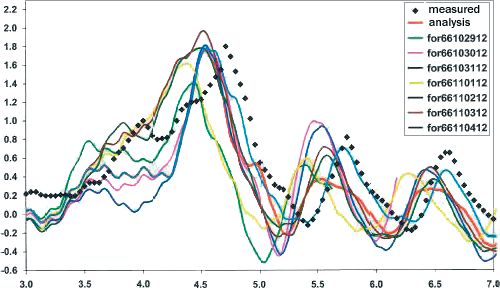
404                                                                 L. Cavaleri et al.

Figure 5. Left panel: the oceanographic tower of ISMAR located 15 km offshore the Venetian littoral (see Figure 1). Right panel: the tower after the storm
of 22 November 1979. The second floor, corresponding to the right extending platform, is shown.

severe damage to the superstructures of the oceanographic  Weather Forecasts Re-Analysis, see Uppala et al. (2005)),
tower (see Figure 5) located in the northern Adriatic Sea, or have been produced using the tools developed by the
15 km offshore the Venetian coast in a 16-metre depth.     ECMWF ERA group. Aiming at a better resolution than
The tower was, and is, manned by ISMAR, the Institute      the related T159 truncation level corresponding to about
of Marine Sciences established in Venice by the Italian    125 km resolution, we have repeated the analysis with
National Research Council after the 1966 storm. Because    T511, corresponding to about 40 km resolution. We have
of the consequent lack of power, no measured wave data is  used the 31R1 version of the ECMWF meteorological
available. The only oceanographic instrument that survived,model, operational at the time when we carried out our
barely but sufficiently, the storm and provided useful dataexperiments. For both the considered storms, a sequence
was a mechanical tide gauge with its recording unit locatedof analyses was done at 12-hour intervals, beginning ten
                                                           days before the date of the storm peak. Starting from
on the second floor of the tower, the one shown in the right
                                                           each analysis, we have generated a series of ten-day
panel of Figure 5. Its location just behind one of the tower
legs shielded it from the highly directional sea. Together forecasts, still with T511, saving the model output fields
with the contemporary sea-level data from the tide gauges  at 3-hour intervals. Including the initial analysis fields,
at the jetty ends, the tower data provided evidence of a   these forecast fields constitute the initial and boundary
                                                           conditions for the limited-area forecasts made with the
sustained wave set-up at the coast reaching more than 40 cm.
(Wave set-up is the increase of sea level in the shore areaBologna Limited Area Model (BOLAM, see below) and
due to the horizontal flux of momentum associated with     provide the meteorological forcing to drive the surge and
wind waves and their breaking when moving into shallow     wave oceanographic models.
areas; see Longuet-Higgins and Stewart (1964) and Bowen       There is a difference between the simulations with the
et al. (1968) for a complete description of the process.)  surge and the wave models. As seen in Figure 1, the narrow
Bertotti and Cavaleri (1985) provide a full discussion of  connection to the Mediterranean Sea at the southern end
                                                           of the Adriatic basin ensures that the wave conditions,
the case. Given that the outer end of the jetty, where the
                                                           particularly in its northern part, depend almost entirely
reference coastal tide gauge is located, protrudes more than
                                                           on the waves generated within the basin. Hence for our
2 km into the sea and the water depth at its end is more than
                                                           present purposes the memory of the system is relatively
6 metres, a much higher set-up was present at the coast.
                                                           short. This is not the case with the surge conditions. The
   Notwithstanding the lack of recorded data, a conservative
                                                           sea level at the Strait of Otranto affects the whole Adriatic
estimate of the maximum wave height at the tower can be    Sea, and thus it is necessary to model the circulation in the
derived from the fact that the tower suffered substantial  whole Mediterranean Sea to have a proper storm surge
damage up to about 9 m above the mean sea level.           simulation. The related response time and memory of
Taking tide into consideration together with the nonlinear the system being much longer than in the wave case, we
character of these extreme waves leads to an estimated     started the surge simulation one month in advance. This
maximum height of the order of 12 m, practically in or     required a month of meteorological data that, for the time
close to breaking conditions. Bertotti and Cavaleri (1985) intervals preceding the already considered ten-day forecasts
provide a full description of the storm and related set-up.at T511 resolution, was derived directly from the ERA-40
                                                           analysis.
4. Methodology                                                The accuracy of the surface wind fields thus obtained
                                                           was not good enough for the wave and surge modelling,
4.1. The meteorological simulation models                  both being very sensitive to small errors of the driving
                                                           wind fields. Indeed (Cavaleri and Bertotti, 1997, 2006) a
All meteorological simulations have been started from ERA- direct application of the ECMWF winds in the Adriatic
40 data (ERA is the European Centre for Medium-Range leads to significant wave heights too low by several tens
            Copyright
                      c 2010 Royal Meteorological Society                                  Q. J. R. Meteorol. Soc. 136: 400–413 (2010)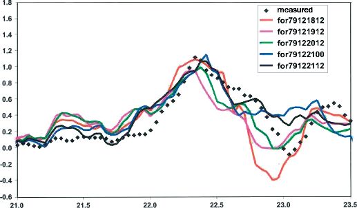
Predictability of Extreme Events in the Adriatic                                         405

of percent. This problem was addressed in two different          runs on an unstructured grid that in the present case becomes
ways. On the one hand, following Cavaleri and Bertotti           progressively denser entering the Adriatic and approaching
(1997, 2006), we have enhanced the ECMWF 10 m wind               the main target area, i.e. moving towards its upper end.
speed over the Adriatic by a constant coefficient. The wind      Note that the SHYFEM grid includes also the lagoon, a
speed over the Mediterranean has been enhanced according         50 × 10 km area on the border of the sea, where Venice is
to the calibrations derived within the project MEDATLAS          located (see Figure 1). A complete description of the model
(Cavaleri and Sclavo, 2006). On the other hand, we have          is given by Umgiesser et al. (2004).
made use of a higher-resolution meteorological model                For the estimate of the wave conditions we used the
nested into the ECMWF one. It is essential to stress that        WAM model (Wamdi Group, 1988; Komen et al., 1994), a
the first approach has not been done ad hoc for these tests,     well established third-generation model amply described
but is a well established and quantified procedure derived       in the literature. It is a spectral model based on a
from long-term tests, regularly applied in the wave (Bertotti    purely physical description of the processes involved in
and Cavaleri, 2009) and surge (Canestrelli and Zampato,          the generation/evolution/dissipation/advection of the ocean
2005) operational forecast systems in the Adriatic Sea. The      wave field. WAM has been integrated with a geographical
correction coefficient in the Adriatic, suitable for sirocco     grid at 1/8 degree resolution, about 14 × 10 km in latitude
storms, depends on the resolution of the meteorological          and longitude respectively. The grid covered the whole
model. It was derived by extensive comparisons of both           Mediterranean Sea when used with the ECMWF winds. It
the wind and associated wave fields against scatterometer,       was limited to the Adriatic Sea when used with the BOLAM
altimeter and buoy data. While we can expect the correction      winds as input. As expected, some direct tests showed
coefficient to vary in space and with the kind of storm, for     that this limitation did not have any impact on the wave
the oceanographic conditions in the northern part of the         conditions in the northern part of the basin.
basin and sirocco storms, a single coefficient turned out to        The WAM and SHYFEM runs have been done for
be a realistic and satisfactory solution. The value 1.35, the    both the ECMWF and BOLAM wind sources. The
one pre-evaluated for the T511 resolution, was used for the      meteorological and the two oceanographic models have been
present tests.                                                   run independently. Lionello et al. (1998, 2003) made several
   As mentioned above, the other approach to cope with           tests on the implications of considering a fully coupled
the problems related to the relatively low resolution of         atmosphere–waves–circulation, including surge, system.
the global meteorological model is to use a nested higher-       Their results suggest that the atmosphere–ocean coupling
resolution one (Jung et al., 2006; Rotach et al., 2009).         is relevant, for whatever waves and surge are concerned,
This was done using a two-step high-resolution limited-area      in areas with a strong air–sea temperature difference. As
model based on the BOLAM model developed at the Institute        also verified from the meteorological data, this was not the
of Atmospheric Sciences and Climate (ISAC) (Buzzi et al.,        case with the warm southerly sirocco winds. As for the
1994; Malguzzi and Tartaglione, 1999; Zampieri et al., 2005),    wave–surge coupling, we point out that, although relevant
run with a 0.18 degree resolution grid (father), covering the    for Venice (with the only exception of a zone very close
area from Portugal to Greece, and a nested grid at 0.06          to the coast) the depth variation associated with the surge
degree (son), centred over the Adriatic Sea. All the BOLAM       is negligible with respect to the local depth. Therefore, as
runs, done in forecast mode (i.e. using the forecasts as         verified also by some direct tests, the implications of coupling
lateral boundary conditions), extended till 1200 UTC of 5        can be judged not relevant for our present results.
November 1966 and 23 December 1979, respectively, with              For the purposes of this paper the tide results are reported
a maximum range of 72 hours. The initial and boundary            at the Salute tide gauge at the border of the Venice area. The
conditions of the father were provided by the ECMWF T511         wave results correspond to the position of the oceanographic
analyses and forecasts discussed above. Such forecasts were      tower (see Figure 1), 15 km offshore, in 16 metres of depth.
used also for the surge runs to fill the surface wind fields
from Greece up to the eastern border of the basin. For the       5.     Results for the November 1966 case
forecasts starting before 1200 UTC of 2 November 1966 and
20 December 1979, the BOLAM runs were started in any case        After a general picture of the storm, we discuss first the
at these times, using as initial conditions the corresponding    meteorological, and then the oceanographic results.
ECMWF T511 forecasts. It is important to stress, also for the       The ECMWF ERA-40 analyses of 10 m enhanced wind
subsequent evaluations, that, at variance with the ECMWF         fields over the Adriatic Sea at 1200 and 1800 UTC on 4
fields, no correction was imposed or attempted on the            November are shown in Figure 6. The intense sirocco wind
BOLAM wind fields. In this respect our aim was to verify if      blowing over the whole basin is clearly represented, with
the quality of the results obtained with the higher resolution   peak wind speeds at 1200 UTC, in front of Venice, higher
of the BOLAM inner grid would have been good enough to           than 28 m/s. The wave conditions follow accordingly, and
overcome the problems associated with the use of a global        their peak is shown in Figure 7. Offshore the northern coast,
model in an enclosed basin.                                      in the area with the highest wind speed, the significant wave
                                                                 height Hs was estimated to exceed 8 m. This value is fully
4.2.   The oceanographic simulation models                       consistent with the damage inflicted by the storm to the
                                                                 jetties (see section 3).
The general circulation and sea-level distribution over the
whole Mediterranean Sea, and in particular the surge             5.1.    Meteorological models
in the Adriatic Sea, were estimated using SHYFEM, a
three-dimensional (3D) finite elements model developed           Concerning the evolution of the storm, Figure 6(b) shows
at ISMAR and used here in its 2D version. SHYFEM is              the passage of the cold front, as represented by the ECMWF
a shallow-water, hydrostatic, primitive equation model. It       analysis, over the northern part of the basin, indicated by a
          Copyright
                    c 2010 Royal Meteorological Society                      Q. J. R. Meteorol. Soc. 136: 400–413 (2010)
406 L. Cavaleri et al.
(a) (b)
16
16
16
16
Figure 6. Wind speed distribution at 10 m height over the Adriatic Sea at (a) 1200, (b) 1800 UTC 4 November 1966 according to the T511 ECMWF
analysis. Isotachs at 4 m/s intervals.
Figure 7. Distribution of wave heights on the Adriatic Sea at 1200 UTC Figure 8. Wind speed distribution at 10 m height over the Adriatic Sea at
4 November 1966 according to the T511 ECMWF analysis. Isolines of 1200 UTC 4 November 1966 according to the BOLAM forecast initiated
significant wave height at 1 metre intervals. Maximum values are above 48 hours in advance. Isotachs at 4 m/s intervals.
8 m, just offshore of Venice at the north-western end of the basin.
for what concerns also the impact on the oceanographic
sudden shift of the wind direction, associated with a speed component, as discussed below.
drop in the cold sector where the direction is from west to Figure 8 shows the corresponding wind peak conditions
southwest. This wind pattern associated with the cold front forecast by the 0.06 degree resolution BOLAM run initialized
is consistent with the pre-frontal low-level jet character of 48 hours in advance. Overall, there is a good agreement
the sirocco wind in this event. In practice, the frontal passage between the ECMWF 10 m wind analysis (Figure 6(a)) and
coincided with the end of the meteorological storm over the the BOLAM (uncorrected) forecast fields. However, some
Adriatic. The timing of the frontal passage in the ECMWF local, relevant differences are present in the most northerly
analysis of Figure 6 (10 m wind speed corrected with the same part of the basin. Consistent with the analysis shown in
coefficient as applied to the forecasts) is also consistent with Figure 6(a), the corresponding ECMWF 48-hour forecast
the position of the cold front subjectively analysed by Fea (not shown) places the area of maximum wind speeds in
et al. (1968) at 1200 UTC (Figure 1) and with the data from front of Venice. On the contrary, due to the fact that the
the Venice unofficial anemometer mentioned in section 3, BOLAM forecast overestimates the propagation speed of the
that pinpointed between 1600 and 1700 UTC as the time the cold front to the east, in this high-resolution forecast the area
cold front passed over the town. Therefore, the relevance of most intense wind speeds is shifted towards the east coast
of a correct estimate of the frontal propagation is evident of the basin, with substantially lower wind speeds in a large
Copyright
c 2010 Royal Meteorological Society Q. J. R. Meteorol. Soc. 136: 400–413 (2010)Predictability of Extreme Events in the Adriatic 407
Figure 9. Time history of the sea level in Venice according to recorded and model data, the latter both as analysis and forecasts initialized at the indicated
times (all 1200 UTC). Input wind fields according to the T511 ECMWF analysis. Time scale: days of November 1966. Height scale: metres.
area in front of Venice. This has limited consequences on Table I. Performance of the surge model using ECMWF and BOLAM
winds.
the local computed wave heights (map not shown), as these
are the results of space and time integrals of the wind fields
along the basin. However, this turned out to be relevant for ECMWF BOLAM
the evaluation of the surge, as will be discussed below.
sea level time sea level time
5.2. Oceanographic results (cm) (hour) (cm) (hour)
29.12 −42 −7
The evolution of the observed meteorological surge, of the
astronomical tide and the resulting sea level are shown in 30.00 −12 5
Figure 3. Remember the true present mean sea level (see 30.12 −7 −4
footnote) and note the negative astronomical tide (−11 cm) 30.00 −72 −6
at the time of the peak. Had the storm hit five hours in 31.12 +2 −5 −60 −2
advance, the flood could have been up to 34 cm higher. For 01.00 +39 −2
a town living between 0.5 and 1.0 m above the present mean 01.12 −21 −8 −60 −9
sea level, this is a result of concern. 02.00 +29 −5
Figure 9 shows the measured evolution of the sea level in 02.12 −5 −5 −46 −6
Venice throughout the storm, the modelled evolution using 03.00 −75 −9 −120 −2
the ECMWF analysis wind fields and the corresponding 03.12 +14 −5 −42 −7
ECMWF forecasts, initialized using the 1200 UTC data 04.00 +46 −2
from 1, 2, 3, up to 6 days in advance (for clarity we have 04.12 −6 −4
not included in this figure the results of the intermediate AN −5 −4
0000 UTC forecasts). Although underestimated in the early
phases of the surge and anticipated by a few hours on the Left column: forecasts initialized at different dates and times, October
day of the peak, all the forecasts clearly show the expected and November 1966. AN is ECMWF analysis. Differences, in cm, between
the peak model values and recorded ones. The time columns report the
surge, usefully quantified up to day 5 in advance, with only time shift, in hours, of the forecast peaks compared with observations (a
a partial underestimation from day 6. Note that Figure 9 negative sign indicates an anticipation of the peak by the forecast).
shows sea levels, which implies, for the mentioned phase
difference between astronomical and surge peaks, that the
timing of the peak of the storm was also, for most forecasts, values were left unchanged. Table I shows that for most of
remarkably correct. the cases there is a phase difference, negative on the average,
Let us now focus on the peak of the storm surge, which, i.e. representing early surge and forecast peak, of only a few
for all practical purposes, is one of the key variables that hours for forecasts up to 144 or 168 hours in advance. It is
describe the event. To facilitate a direct comparison, the easy to see that in general the forecasts based on the 0000
differences between the level and time of the peak values of UTC data are less accurate than the 1200 UTC ones. This
the official record and those estimated using the ECMWF is particularly the case on 30 October and on 3 November,
analysis and all the ECMWF and BOLAM forecasts are listed the latter being more remarkable because issued less than
in Table I. When comparing the ECMWF with the BOLAM 36 hours before the event.
results, it should be borne in mind that, as mentioned To understand better the origin of this miss we need first
in section 4, while the ECMWF wind speed values were to understand the crucial role of the wind conditions in the
enhanced using a multiplying factor, the BOLAM speed upper part of the basin. The difficulty of a surge forecast is
Copyright
c 2010 Royal Meteorological Society Q. J. R. Meteorol. Soc. 136: 400–413 (2010)408 L. Cavaleri et al.
would be no flood at all. Also the forecast wave heights
are much lower. The interpretation of the nature – not of
the cause – of the meteorological forecast error is shown
in Figure 11. Here we compare the analysis wind field of
1200 UTC 4 November, the peak of the storm, with the
corresponding forecast started 36 hours in advance. Clearly
the forecast has anticipated the passage of the cold front.
A comparison with its actual position 6 hours later in
Figure 6(b) suggests a time shift of about 9 hours. The
matter becomes clear when we look at the distribution of
Figure 10. Longitudinal section, along its main axis, of the sea-level
the surge in Figure 10. Due to the mentioned increase of
distribution in the Adriatic Sea (see Figure 1) at the peak of the flood at the sea-level spatial gradients with decreasing depth, and
1200 UTC 4 November 1966. because of the wind distribution (see Figure 6(a)), most
of the surge was concentrated in the upper part of the
basin, in practice in front of Venice. The anticipation of
well exemplified in Figure 10, where we see a section of the the frontal passage completely changed the wind speed and
sea-level distribution along the main axis of the Adriatic at direction in this area at the crucial moment when the surge
the time of the peak of the surge. For a given surface stress, the was mounting. The result is the drastic underestimate seen
increased spatial gradient with decreasing depth leads to the in Table I. This highlights how critical the surge forecasts
surge just in front of the Venice coast. It follows that even lim- can be, depending on small shifts in time and position
ited differences of the wind field in this area, e.g. a shift of the of the forcing fields. To a lesser extent because of their
location of maximum strength with a decrease of the wind stronger dependence on the overall field, the wave heights
speeds in the shallower area, can substantially alter the surge. also showed locally a substantial decrease. This was probably
This explains why the maximum sea-level values derived associated with the local breaking (steep waves moving
from the BOLAM forecasts are lower than the ECMWF ones into shallower depths) and absence of direct forcing by
(and than the ‘official’ peak) by about 40 cm. As discussed wind.
above and seen in Figure 8, the area of maximum wind The question is how this was possible. Note that the
speeds in BOLAM is adjacent to the Croatian coast, leaving previous and following forecasts, initialized at 1200 UTC 2
substantially lower wind speeds in front of the northern and 3 November respectively, pinpoint the storm exactly.
coast, where (Figure 10) most of the surge is concentrated. Something similar happened on 15–16 October 1987, when
Given the comparison between the ECMWF and BOLAM an exceptional Atlantic storm hit Brittany, the south of the
surge results in Table I, this seems to be a characteristic of United Kingdom and the Channel area. A good description
all the BOLAM forecasts analysed in this 1966 case-study. of the event and discussion of the forecasts was given, among
Having clearly in mind the role of the wind in the others, by Burt and Mansfield (1988) and Morris and Gadd
upper part of the basin, we can now go back to the wrong (1988). The storm had been predicted in the previous days,
forecast issued 36 hours before the 1966 event. For clarity but it was practically absent on the maps issued during the
reasons in Figure 9 we have shown only the surge forecasts last period before the event. The later analysis showed this
issued at 1200 UTC, while all the results are reported in was due to a wrong ship report, one of the few available in the
Table I. Indeed the forecast starting at 03.00 (0000 UTC area at the crucial moment. Thus, one possible explanation of
3 November) is not only substantially underestimated, but the poor prediction started at 0000 UTC of 3 November 1966
for all practical purposes according to this forecast there could be the poor quality, and/or the lack of enough data to
(a) (b)
Figure 11. Left panel: distribution of the 10 m wind field (analysis) over the Adriatic Sea at 1200 UTC 4 November 1966 (see Figure 6(a)). Right panel:
corresponding field according to the forecast initialized 36 hours in advance.
Copyright
c 2010 Royal Meteorological Society Q. J. R. Meteorol. Soc. 136: 400–413 (2010)Predictability of Extreme Events in the Adriatic 409
Table II. Performance of the wave model using ECMWF and BOLAM Table III. As Table II, but for the storm of December 1979.
winds.
ECMWF BOLAM
ECMWF BOLAM
Hs (m) time (hour) Hs (m) time (hour)
Hs (m) time (hour) Hs (m) time (hour)
17.00 4.8 −3
29.12 5.3 −6 17.12 6.5 −3
30.00 1.6 −18 18.00 6.8 0
30.12 4.7 0 18.12 7.2 −3 4.9 0
31.00 3.8 −6 19.00 6.6 0
31.12 5.3 0 4.4 +3 19.12 6.3 −3 4.8 0
01.00 7.3 +3 20.00 6.2 −3
01.12 6.2 −6 5.2 −6 20.12 5.9 0 4.4 0
02.00 7.2 0 21.00 6.4 0 4.9 0
02.12 7.3 −3 6.8 −6 21.12 6.4 0 4.9 0
03.00 3.8 −12 2.7 −12 22.00 6.5 0
03.12 7.0 −3 7.2 −6 AN 5.6 –
04.00 7.3 +3
AN 6.3 –
Left column: forecasts initialized at different dates and times, October and
November 1966. AN is ECMWF analysis. Hs is the maximum significant the wave results. The waves obtained using the enhanced
wave height (m) estimated at the position of the oceanographic tower ECMWF winds are higher and appear to be more consistent
(see Figure 1 for its position and Figure 6 for the implications). The time with the damage seen in Figure 5. Because the wave heights
columns report the time shift, in 3-hour steps, of the forecast wave peaks
compared with the analysis (a negative sign indicates an anticipation by depend on the overall situation on the basin, we derive that
the forecast). (see also the discussion in section 7) the enhanced ECMWF
wind fields are more representative of the situation in the
Adriatic Sea. However, Table IV shows that the BOLAM
produce an accurate analysis of that time. We attempted a surge peak values fit the measured one better. Following our
deeper analysis in this direction (Cardinali et al., 2007; Kelly
previous argument in section 2 and section 5, this suggests
et al., 2007), but no definite conclusion was reached.
too-high ECMWF wind speeds in the area in front of Venice.
In general, the lower quality of the 0000 UTC forecasts can
Indeed a direct inspection (not shown) of the ECMWF and
be expected to be associated with that of the corresponding
BOLAM surface wind maps in the hours just before the peak
analysis. We speculate that in turn this might be related to
shows the former wind speeds to be on average 20–30%
the lack, or to a lower quality, of the data available at 0000
higher than the latter ones. This conclusion is supported by
UTC compared to that recorded at 1200 UTC.
The results of the wave simulations are summarised in a direct comparison of the values reported in Table V with
Table II. Apart from the already mentioned forecasts started the data from the (mechanical) anemometer on-board the
at 0000 UTC of 3 November and of 30 October, the values tower. Seen on the left, the ECMWF data are too high for
confirm that also for the waves the situation was predictable practically the whole duration of the storm. Focusing on the
up to six days in advance. Note that the BOLAM and value at the peak of the storm (0600 UTC 22 December), we
ECMWF models give more consistent (between the two compare on the right the ECMWF and BOLAM peak values
models) forecasts of the wave fields (Table II) than of the sea from the forecasts issued at different dates and times. With
level (Table I). The reason is that the wave conditions in the respect to the 16.4 m/s measured value, the ECMWF wind
northern part of the basin depend on the whole wind fields speeds are too high, while, starting from the 19 December
along the Adriatic. In the respect, the ECMWF and BOLAM 1200 UTC forecast, the BOLAM values have practically no
average wind fields are much more similar to each other, bias.
and the shift towards the east of the BOLAM peak area does These results indicate that, while in the Adriatic Sea the
not have the same consequences as for the surge forecasts. wind field is generally correct for ECMWF but it is too weak
for BOLAM, in front of Venice the local wind speed is too
6. Results for the December 1979 case high for ECMWF but practically correct for BOLAM. The
quality of the surge forecasts followed accordingly.
Figure 12 shows the time series of recorded and forecast
surge in Venice modelled using the BOLAM winds. Rather 7. Discussion and conclusions
than also plotting the ECMWF results, peak values computed
using both model winds are contrasted in Table III. Table III The performance of state-of-the-art meteorological and
indicates that both forecasts have very good timings, with oceanographic numerical systems in predicting the sea state
a maximum shift of less than four hours, reduced to one in the Adriatic Sea during intense storms is assessed, also in
or two for initial conditions in the few days preceding the the case of past storms, when the amount of data available
flood. was much lower than today. The key issue that has been
The comparison between the ECMWF and BOLAM wave addressed by this study is whether severe events such as
heights and surges at the measuring tower offshore Venice those that affected Venice in 1966 and in 1979 could have
confirms again the crucial role of the wind in the shallow been predicted if the forecasting models/data available now
area in front of Venice. Let us consider first in Table III had been present at that time.
Copyright
c 2010 Royal Meteorological Society Q. J. R. Meteorol. Soc. 136: 400–413 (2010)410 L. Cavaleri et al.
Figure 12. Time history of the sea level in Venice according to recorded and model data, the latter as forecasts initialized at the indicated times. Input
wind fields according to the BOLAM model initialized 36 hours in advance. Time scale: days of December 1979. Height scale: metres.
Table IV. As Table I, but for the storm of December 1979. comes from Canestrelli and Zampato (2005), see also Bajo
et al. (2007), who discussed statistics of the tide forecast
ECMWF BOLAM system operational in Venice, and showed that operational
forecasts of ‘average’ sea-state conditions issued two days in
sea level time sea level time advance are, in general, reliable. To our knowledge, there
(cm) (hour) (cm) (hour) is no evidence in the public literature of the quality of
operational forecasts of the sea state in the Adriatic Sea in
17.00 +14 −4 cases of ‘extreme’ conditions. The second piece of evidence
17.12 +57 −4 comes from a study of the predictability of severe weather
18.00 +54 +1 events that affect the Italian Peninsula. In fact, Grazzini
18.12 +70 0 −3 0 (2007) showed that events as exceptional as those of 1966
19.00 +58 +4 and 1979 are associated with large-scale synoptic conditions
19.12 +25 −2 −16 0 that are easier to predict. The two cases discussed in this
20.00 +30 +1 work support this conjecture. Thus, although less intense sea
20.12 +32 +1 −11 +1 conditions might be predictable only for up to few days in
21.00 +42 +1 +4 +2 advance, extreme cases associated with larger-scale synoptic
21.12 +43 +1 −6 +2 forcing could be predictable with longer lead times.
22.00 +47 +2 The comparison between the performance of the ECMWF
and BOLAM models has given some useful indications on
AN +19 +1
the design of a future, more skilful operational system for
the prediction of oceanographic states. It is by now amply
accepted also in the meteorological community (Janssen,
Although it is impossible to draw statistically significant 2008) that the results of an advanced wave model are one
conclusions from only two cases, this study has shown of the best indicators of the overall quality of the driving
that, at least for these two events, state-of-the-art numerical wind fields. This is true not only over the oceans, but also,
models of the atmosphere and the ocean would have been and more so, over an enclosed sea where limited shifts or
capable of predicting the storms that affected Venice and changes of the meteorological pattern may lead to drastic
the northern Adriatic Sea several days in advance. The changes over the area of interest. The same sensitivity is felt
accuracy obtained for the two events in terms of intensity of by the limited-area meteorological models that, with their
surface winds, surge level, wave height and timing, although capability to carve out details not visible in a global model,
lower for the earlier case, can be considered sufficient for are highly sensitive to small errors of the father model.
issuing different types of alert at different stages in both The underestimate of wind speed by a model, especially in
cases. These results, combined with the fact that nowadays enclosed seas, is dependent on its resolution. Accordingly,
10–100 times more data are available, forecast models the BOLAM model has provided substantially higher wind
have been continuously improving, and more sophisticated speeds than the ECMWF one, although, according to our
data assimilation systems are used, suggest that, should results, still somehow too low. An objective, independently
comparable events happen again, valuable forecasts could pre-defined enhancement of the ECMWF wind speeds
be made available to the public and acting authorities a-few- brought them to a quality level sufficient for practical
to-several days in advance, well in time for any necessary purposes.
action. Two pieces of evidence, and the results discussed in Given the meteorological predictability, the correspond-
this work, support this conclusion. The first piece of evidence ing oceanographic one depends on the specific situation. In
Copyright
c 2010 Royal Meteorological Society Q. J. R. Meteorol. Soc. 136: 400–413 (2010)Predictability of Extreme Events in the Adriatic 411
Table V. Comparison between recorded and ECMWF analysis wind speeds at the position of the oceanographic tower (see Figure 5).
date time Record ECMWF analysis date time ECMWF forecast BOLAM forecast
21 18 12.8 12.4
21 13.3 15.2
22 00 11.3 17.1 18 12 22.3 17.0
03 10.8 17.2 19 12 20.0 16.5
06 16.4 18.1 forecast 20 12 19.7 16.2
09 – 18.3 21 00 18.6 16.6
12 13.8 18.5 21 12 18.2 16.3
15 13.3 16.9
18 8.7 10.4
Values in m/s. Dates and times shown in the first two columns. The period is December 1979. Right part: focusing on the value at 0600 UTC 22
December, comparison with the corresponding forecast values using ECMWF and BOLAM winds. Forecasts initialized at the indicated dates and
times.
the case of the Adriatic Sea, and also in the more general reader is referred also to Buizza et al. (2007) and Palmer
case, waves depend on the wind distribution over the overall et al. (2007) for further discussions of the performance of
basin of interest. Therefore limited changes in the wind dis- the ECMWF EPS in predicting weather conditions. Work to
tribution are not likely to have drastic consequences. This is assess the performance of ECMWF probabilistic forecasts of
not the case with storm surges, the more so the shallower the sea state in the Adriatic Sea is in progress, and will be
the water. Because most of the surge is concentrated in the reported in due course.
lower depth areas, limited variations of the wind field in this In conclusion, the implications of this work on the future
zone could lead to large differences in the results. prediction of sea-state events such as the ones that affected
An example is given by the wrong forecast issued on the Venice in 1966 and 1979 are the following:
basis of the data available on 3 November 1966. Comparing
(1) Notwithstanding the substantial lack of data that
this situation to a similar miss which happened on the
characterised those early years, the application of the
French–English coasts in October 1987, we have tried to
present tools (computers and models) to the data of
trace back the origin of the mistake. However, the kind
1966 and 1979 has shown that in principle useful
and structure of the data available for 1966 did not allow
forecasts would have been possible up to several days
any conclusion to be reached. The relevant question is
in advance. One of the reasons why the prediction of
whether such a miss could also happen today, 20 years
this (extreme) type of event could be easier that the
after the failure of 1987. We tend to think that the prediction of ‘average’ states is that extreme sea-state
present enormous amount of data and the keen analysis conditions are associated with large-scale synoptic
of their consistency done before and during assimilation forcing, which makes them more predictable than
should exclude that one or a few isolated wrong data small-scale, local phenomena.
could drastically affect the analysis, hence the forecast. (2) Particularly in enclosed seas, the oceanographic model
Unfortunately, after 1987, models struggled, for example, results are very sensitive to errors in the input
to correctly predict the development of two severe storms wind fields. Especially in shallow-water areas, this
that hit France and north-central Europe in December 1999 is more the case for surge than wave results, the latter
(Buizza and Hollingsworth, 2002). Should a storm like this depending more on the general distribution of the
occur over the Mediterranean, it could cause single forecasts winds on the considered basin.
to miss the prediction of severe sea-state conditions a few (3) The ECMWF wind speeds, as representative of the
days ahead, thus making it impossible to issue warnings a global models, turn out to be too low in enclosed seas.
few days before the occurrence of the event. Much better results, although somehow still lower
Is there a way to further improve and reduce the forecast than the truth, are obtained with high-resolution
uncertainty? Buizza and Hollingsworth (2002) showed that limited-area meteorological models. For a given basin
for the two storms of December 1999 a probabilistic an alternative approach is to use suitable enhancement
approach to the prediction of severe events led to early coefficients for the global model wind speeds, derived
indications of possible severe storm occurrence. They from long-term comparison between atmospheric
concluded that a probabilistic, ensemble-based approach and wave model results and measured data in the area
to weather prediction gives users valuable forecasts about of interest. Depending on the geometry and orography
one day before single forecasts, and illustrated that the of the basin, these coefficients may depend on the
ECMWF Ensemble Prediction System (EPS) is an extremely type of storm. They depend also on the resolution
valuable tool for assessing quantitatively the risk of severe of the meteorological model. Results have indicated
weather and issuing early warnings of possible disruptions. that dynamical downscaling of the large-scale weather
Saetra et al. (2004) compared the performance of EPS-based fields with a limited-area model could improve the
probabilistic and single forecasts of sea waves and winds sea-state prediction, especially of the wave field.
for about 2.5 years, and concluded that EPS probabilistic (4) Results so far indicate that a warning system for
forecasts are more valuable for decision makers. A good the Adriatic Sea that includes a high-quality global
example of practical application of the ensemble technique weather model, a high-quality limited-area model
to surge forecasts is given by Flowerdew et al. (2009). The and sea-state and surge models, should provide users
Copyright
c 2010 Royal Meteorological Society Q. J. R. Meteorol. Soc. 136: 400–413 (2010)412 L. Cavaleri et al.
with valuable forecasts up to several days in advance, change on flooding and sustainable river management, RIBAMOD
particularly in the case of severe events. Workshop, Wallingford, 26–27 February 1998. EUR 18287 EN.
European Commission: Luxembourg.
(5) But it should be pointed out that small errors in the De Zolt S, Lionello P, Nuhu A, Tomasin A. 2006. The disastrous storm
initial analysis fields will always be present, e.g. due of 4 November 1966 on Italy. Natural Hazards Earth Syst. Sci. 6:
to possible observation errors. These initial errors 861–879.
may lead to substantial errors in the forecast of Fea G, Gazzola A, Cicala A. 1968. ‘Prima documentazione generale della
situazione meteorological relativa alla grande alluvione del novembre
meteorological situations, and thus to even larger 1966.’ CNR-CENFAM PV 32: 215 pp.
oceanographic errors (see also point (2)). One way to Flowerdew J, Horsburgh KJ, Mylne KR. 2009. Ensemble forecasting of
address this issue is to use a probabilistic approach, storm surges. Mar. Geodesy 32: 91–99.
and thus develop a probabilistic sea-state forecasting Grazzini F. 2007. Predictability of a large-scale flow conducive to
extreme precipitation over the western Alps. Meteorol. Atmos. Phys.
system that includes a global EPS, a limited-area EPS 95: 123–138.
and a sea-state ensemble system. Janssen PAEM. 2008. Progress in ocean wave forecasting. J. Comput.
Phys. 227: 3572–3594.
Work along the lines of this latter point to assess the Jung T, Gulev SK, Rudeva I, Soloviov V. 2006. ‘Sensitivity of
value of the probabilistic forecast of sea states in case of extratropical cyclone characteristics to horizontal resolution in the
‘acqua-alta’ in Venice is under progress, and results will be ECMWF model.’ ECMWF RD Tech. Memo. 485. Available from
ECMWF, Shinfield Park, Reading RG2 9AX, UK (also from
reported in due course. www.ecmwf.int/publications/library).
Kelly G, Thépaut J-N, Buizza R, Cardinali C. 2007. The value of
Acknowledgements observations. I: Data denial experiments for the Atlantic and the
Pacific. Q. J. R. Meteorol. Soc. 133: 1803–1815.
Komen GJ, Cavaleri L, Donelan M, Hasselmann K, Hasselmann S,
We want to thank Graeme Kelly and Sakari Uppala for their Janssen PAEM. 1994. Dynamics and modelling of ocean waves.
help with generating higher-resolution re-analyses of the Cambridge University Press.
situations. The original idea of this research, of applying Lionello P, Malguzzi P, Buzzi A. 1998. Coupling between the atmospheric
circulation and the ocean wave field: An idealized case. J. Phys.
the present methods for a posteriori forecasts of storms very Oceanogr. 28: 161–177.
much in the past, was suggested by Tony Hollingsworth. Lionello P, Martucci G, Zampieri M. 2003. Implementation of a coupled
The study has been partially supported by the Consorzio atmosphere–wave–ocean model in the Mediterranean Sea: Sensitivity
Venezia Nuova in relation to the predictability of the big of the short time scale evolution to the air–sea coupling mechanisms.
Global Atmos. Ocean System 9: 65–95.
floods affecting Venice. Longuet-Higgins MS, Stewart RW. 1964. Radiation stresses in water
waves: A physical discussion with applications. Deep-Sea Res. 11:
529–562.
References Malguzzi P, Tartaglione N. 1999. An economical second-order advection
Bajo M, Zampato L, Umgiesser G, Cucco A, Canestrelli P. 2007. A finite scheme for numerical weather prediction. Q. J. R. Meteorol. Soc. 125:
element operational model for storm surge prediction in Venice. 2291–2303.
Estuar. Coast. Shelf Sci. 75: 236–249. Malguzzi P, Grossi G, Buzzi A, Ranzi R, Buizza R. 2006. The 1966
Bertò A, Buzzi A, Nardi D. 2005. ‘A warm conveyor belt mechanism ‘century’ flood in Italy: A meteorological and hydrological revisitation.
accompanying extreme precipitation events over north-eastern J. Geophys. Res. 111: D24106, DOI:10.1029/2006JD007111.
Morris RM, Gadd AJ. 1988. Forecasting the storm of 15–16 October
Italy.’ Proceedings 28th ICAM, The annual Scientific MAP Meeting,
1987. Weather 43: 70–90.
2005, Zadar, extended abstracts. Hrv. Meteorol. Casopis (Croatian
Palmer TN, Buizza R, Leutbecher M, Hagedorn R, Jung T, Rodwell M,
Meteorological Journal) 40: 338–341.
Vitart F, Berner J, Hagel E, Lawrence A, Pappenberger F, Park Y-Y,
Bertotti L, Cavaleri L. 1985. Coastal set-up and wave breaking. Oceanol.
von Bremen L, Gilmour I. 2007. ‘The Ensemble Prediction System:
Acta 8: 237–242.
Recent and ongoing developments. A paper presented at the 36th Session
Bertotti L, Cavaleri L. 2009. Large and small scale wave forecast in the
Mediterranean Sea. Natural Hazards Earth Syst. Sci. 9: 779–788. of the ECMWF Scientific Advisory Committee.’ ECMWF Research
Bowen AJ, Inman DL, Simmons VP. 1968. Wave ‘set-down’ and set-up. Department Technical Memorandum 540, ECMWF, Shinfield Park,
J. Geophys. Res. 73: 2569–2577. Reading, RG2 9AX, UK.
Buizza R, Hollingsworth A. 2002. Storm prediction over Europe using Pirazzoli PA, Tomasin A. 2003. Recent near-surface wind changes in
the ECMWF Ensemble Prediction System. Meteorol. Appl. 9: 289–305. the central Mediterranean and Adriatic areas. Int. J. Climatol. 23:
Buizza R, Cardinali C, Kelly G, Thépaut J-N. 2007. The value of 963–973.
observations. II: The value of observations located in singular-vector- Pugh DT. 1987. Tides, surges, and mean sea-level. John Wiley & Sons:
based target areas. Q. J. R. Meteorol. Soc. 133: 1817–1832. Chichester, New York.
Burt SD, Mansfield DA. 1988. The great storm of 15–16 October 1987. Rotach MW, Ambrosetti P, Ament F, Appenzeller C, Arpagaus M,
Weather 43: 90–114. Bauer H-S, Behrendt A, Bouttier F, Buzzi A, Corazza M, Davolio S,
Buzzi A, Fantini M, Malguzzi P, Nerozzi F. 1994. Validation of a limited Denhard M, Dorninger M, Fontannaz L, Frick J, Fundel F, Germann U,
area model in cases of Mediterranean cyclogenesis: Surface fields and Gorgas T, Hegg C, Hering A, Keil C, Liniger MA, Marsigli C,
precipitation scores. Meteorol. Atmos. Phys. 53: 137–153. McTaggart-Cowan R, Montaini A, Mylne KR, Ranzi R, Richard E,
Camuffo D. 1993. Analysis of the sea surges at Venice from AD 782 to Rossa A, Santos-Muñoz D, Schär C, Seity Y, Staudinger M, Stoll M,
1990. Theor. Appl. Climatol. 47: 1–14. Volkert H, Walser A, Wang Y, Werhahn J, Wulfmeyer V, Zappa M.
Canestrelli P, Zampato L. 2005. Sea-level forecasting at the Centro 2009. MAP D-PHASE: Real-time demonstration of weather forecast
Previsioni e Segnalazioni Maree (CPSM) of the Venice Municipality. quality in the Alpine region. Bull. Am. Meteorol. Soc. 90: 1321–1336.
Pp 85–97 in Flooding and environmental challenges for Venice and its Saetra Ø, Hersbach H, Bidlot J-R, Richardson DS. 2004. Effects of
lagoon: State of knowledge, Fletcher C, Spencer T (eds). Cambridge observation errors on the statistics for ensemble spread and reliability.
University Press: Cambridge, UK. Mon. Weather Rev. 132: 1487–1501.
Cardinali C, Buizza R, Kelly G, Shapiro M, Thépaut J-N. 2007. The value Tomasin A. 2005. Forecasting the water level in Venice: Physical
of observations. III: Influence of weather regimes on targeting. Q. J. background and perspectives. Pp 71–78 in Flooding and environmental
R. Meteorol. Soc. 133: 1833–1842. challenges for Venice and its lagoon: State of knowledge, Fletcher CA,
Cavaleri L, Bertotti L. 1997. In search of the correct wind and wave fields Spencer T (eds). Cambridge University Press.
in a minor basin. Mon. Weather Rev. 125: 1964–1975. Umgiesser G, Melaku Canu D, Cucco A, Solidoro C. 2004. A finite
Cavaleri L, Bertotti L. 2006. The improvement of modelled wind and element model for the Venice lagoon: Development, set up, calibration
wave fields with increasing resolution. Ocean Engineering 33: 553–565. and validation. J. Mar. Sys. 51: 123–145.
Cavaleri L, Sclavo M. 2006. The calibration of wind and wave model data Uppala SM, Kållberg PW, Simmons AJ, Andrae U, da Costa Bechtold V,
in the Mediterranean Sea. Coastal Engineering 53: 613–627. Fiorino M, Gibson JK, Haseler J, Hernandez A, Kelly GA, Li X,
Cecconi G, Canestrelli P, Corte C, Di Donato M. 1999. ‘Climate Onogi K, Saarinen S, Sokka N, Allan RP, Andersson E, Arpe K,
record of storm surges in Venice.’ Pp 149–156 in Impact of climate Balmaseda MA, Beljaars ACM, van de Berg L, Bidlot J, Bormann N,
Copyright
c 2010 Royal Meteorological Society Q. J. R. Meteorol. Soc. 136: 400–413 (2010)You can also read