Overexploitation, Recovery, and Warming of the Barents Sea Ecosystem During 1950-2013
←
→
Page content transcription
If your browser does not render page correctly, please read the page content below
ORIGINAL RESEARCH
                                                                                                                                      published: 17 September 2021
                                                                                                                                    doi: 10.3389/fmars.2021.732637

                                            Overexploitation, Recovery, and
                                            Warming of the Barents Sea
                                            Ecosystem During 1950–2013
                                            Torstein Pedersen 1* , Nina Mikkelsen 1,2 , Ulf Lindstrøm 1,2 , Paul E. Renaud 3,4 ,
                                            Marcela C. Nascimento 1 , Marie-Anne Blanchet 5† , Ingrid H. Ellingsen 6 , Lis L. Jørgensen 2
                                            and Hugues Blanchet 3,7
                                            1
                                              Department of Arctic and Marine Biology, Faculty of Biosciences, Fisheries and Economics, UiT The Arctic University of
                                            Norway, Tromsø, Norway, 2 Norwegian Institute of Marine Research (IMR), Tromsø, Norway, 3 Akvaplan-Niva AS, Fram
                            Edited by:
                                            Centre for Climate and the Environment, Tromsø, Norway, 4 University Centre in Svalbard, Longyearbyen, Norway,
                Alistair James Hobday,      5
                                              Norwegian College of Fisheries Science, UiT-The Arctic University of Norway, Tromsø, Norway, 6 SINTEF Ocean, Trondheim,
            Commonwealth Scientific
                                            Norway, 7 Environnements et Paléoenvironnements Océaniques et Continentaux, University of Bordeaux, Bordeaux, France
 and Industrial Research Organisation
                      (CSIRO), Australia
                       Reviewed by:         The Barents Sea (BS) is a high-latitude shelf ecosystem with important fisheries, high
                   Chongliang Zhang,        and historically variable harvesting pressure, and ongoing high variability in climatic
    Ocean University of China, China
                   Nor Azman Kasan,
                                            conditions. To quantify carbon flow pathways and assess if changes in harvesting
   University of Malaysia Terengganu,       intensity and climate variability have affected the BS ecosystem, we modeled the
                              Malaysia
                                            ecosystem for the period 1950–2013 using a highly trophically resolved mass-balanced
                  *Correspondence:
                                            food web model (Ecopath with Ecosim). Ecosim models were fitted to time series
                     Torstein Pedersen
             Torstein.Pedersen@uit.no       of biomasses and catches, and were forced by environmental variables and fisheries
                † Present address:          mortality. The effects on ecosystem dynamics by the drivers fishing mortality, primary
              Marie-Anne Blanchet,          production proxies related to open-water area and capelin-larvae mortality proxy,
   Norwegian Polar Institute, Tromsø,
                              Norway
                                            were evaluated. During the period 1970–1990, the ecosystem was in a phase of
                                            overexploitation with low top-predators’ biomasses and some trophic cascade effects
                  Specialty section:        and increases in prey stocks. Despite heavy exploitation of some groups, the basic
        This article was submitted to
        Marine Fisheries, Aquaculture
                                            ecosystem structure seems to have been preserved. After 1990, when the harvesting
               and Living Resources,        pressure was relaxed, most exploited boreal groups recovered with increased biomass,
              a section of the journal
                                            well-captured by the fitted Ecosim model. These biomass increases were likely driven
         Frontiers in Marine Science
                                            by an increase in primary production resulting from warming and a decrease in ice-
           Received: 29 June 2021
        Accepted: 20 August 2021            coverage. During the warm period that started about 1995, some unexploited Arctic
     Published: 17 September 2021           groups decreased whereas krill and jellyfish groups increased. Only the latter trend was
                              Citation:     successfully predicted by the Ecosim model. The krill flow pathway was identified as
             Pedersen T, Mikkelsen N,
             Lindstrøm U, Renaud PE,
                                            especially important as it supplied both medium and high trophic level compartments,
     Nascimento MC, Blanchet M-A,           and this pathway became even more important after ca. 2000. The modeling results
      Ellingsen IH, Jørgensen LL and
                                            revealed complex interplay between fishery and variability of lower trophic level groups
  Blanchet H (2021) Overexploitation,
       Recovery, and Warming of the         that differs between the boreal and arctic functional groups and has importance for
      Barents Sea Ecosystem During          ecosystem management.
                          1950–2013.
            Front. Mar. Sci. 8:732637.      Keywords: ecosystem dynamics, mass-balance modeling, trophic flows, environmental drivers, sequential
    doi: 10.3389/fmars.2021.732637          depletion, food web, primary production variability

Frontiers in Marine Science | www.frontiersin.org                                 1                                      September 2021 | Volume 8 | Article 732637
Pedersen et al.                                                                                                  Barents Sea Ecosystem Dynamics

INTRODUCTION                                                             capelin, and seabirds (Johannesen et al., 2012; Fauchald et al.,
                                                                         2015; Gjøsæter et al., 2015). Relationships and energetics of major
Fisheries and climate have been emphasized as major drivers of           stocks of top-predators, such as Northeast Arctic cod, minke
energy flows in large marine ecosystems (LMEs) (Araujo and               whales, and harp seals have also changed (Bogstad et al., 2015;
Bundy, 2012; Link et al., 2012), and understanding how these             Fauchald et al., 2015).
drivers interacts and shapes ecosystems is a major challenge                 The change in climatic conditions call for an effort to use
and essential to manage these ecosystems. It is important                and integrate available information to understand the underlying
to investigate how these drivers interplay in high-latitude              drivers for the ecosystem changes, and ecosystem modeling
ecosystems, such as the Barents Sea. The Barents Sea (BS)                is a common tool to synthesize quantitative information into
is intensely exploited and profoundly impacted by climate                a coherent system. This is particularly important in species-
variability. It is characterized by a strong temperature gradient        rich systems with complex (e.g., with considerable advection
with boreal and sub-arctic conditions in the southwest and               and migration) pathways for impact where statistical modeling
high-arctic conditions in the northeast (Loeng, 1991; Smedsrud           may struggle. Previously published food web models of the
et al., 2010), and advected heat, nutrients, and biota, along            BS and Norwegian Sea have been fish-centered with relatively
with seasonally migrating fish, seabirds, and mammals strongly           few lower trophic level groups and benthic invertebrate groups
impact ecosystem structure and production (Hunt et al., 2013).           (Blanchard et al., 2002; Dommasnes et al., 2002; Hansen et al.,
The trophic structure of the BS ecosystem is similar to other            2016; Skaret and Pitcher, 2016; Bentley et al., 2017). Arctic
northern high latitude shelf ecosystems (Gaichas et al., 2009;           and sub-Arctic ecosystems, however, are well-known for the
Eriksen et al., 2017).                                                   strong role of seafloor communities in regulating carbon cycling
    Fisheries has been a major direct driver of marine ecosystems        pathways (K˛edra and Grebmeier, 2021). Based on a dynamic
the past century, affecting structure, function, and diversity           mass-balance model (Ecopath with Ecosim-EwE) and future
(Jackson, 2001; Halpern et al., 2008). The fisheries within the BS       warming scenarios for the Norwegian and the BS, Bentley et al.
have since the 1950s been targeting mainly large gadoid fishes,          (2017) suggested that the biomasses of widely migrating pelagic
such as Atlantic cod (Gadus morhua), haddock (Melanogrammus              species, such as mackerel and blue whiting, are expected to
aeglefinus) and saithe (Pollachius virens) and other demersal            increase with future rising ocean temperature. There is some
fishes, such as Greenland halibut (Reinhardtius hippoglossoides)         evidence that effects of climate variability on the ecosystem in
and redfishes (Sebastes mentella and Sebastes norvegicus), the           the BS is largely through bottom-up effects on lower trophic level
small pelagic fish species capelin (Mallotus villosus) and polar         groups that propagate to higher trophic level groups (Johannesen
cod (Boreogadus saida), and northern shrimp (Pandalus borealis)          et al., 2012; Dalpadado et al., 2014, 2020).
(Gjøsæter, 1998; Nakken, 1998; Hop and Gjøsæter, 2013; Haug                  Fisheries and climate change may act synergistically with each
et al., 2017). Juvenile Atlantic herring (Clupea harengus) was           other and/or with other anthropogenic disturbances (Fogarty
fished within the area from 1950 to 1971 (Toresen and Østvedt,           et al., 2008; Hsieh et al., 2008). Exploited populations may be
2000). Some marine mammals were also heavily exploited up                less resilient to climate variability than unexploited populations
until their protection, such as walrus (Odobenus rosmarus)               due to more truncated age structure and diversity in life
(protected in 1952), polar bear (protected in 1973), and some            history traits (Fogarty et al., 2008; Hsieh et al., 2008). A better
large baleen whales (Nakken, 1998; Weslawski et al., 2000). After        understanding of how exploitation and climate variability
ca 1970, the only mammals harvested in large scale have been             influence the ecosystem dynamics will support management of
minke whales and harp seals (Nakken, 1998).                              marine resources.
    Climate variability may affect marine ecosystems through                 Aggregating species into trophic groups may mask complex
effects on primary and secondary production, fish recruitment            species interactions and influence calculations associated with
variability, growth and shifts of populations distribution range         food webs and interspecific competition (Thompson and
(Nilssen et al., 1994; Ottersen and Loeng, 2000; Fossheim et al.,        Townsend, 2000). Therefore, to analyze trophic interactions and
2015). In the BS, a period of warm climate between 1920 and 1960         impacts of harvesting and climate variability in this study, we
was followed by a cold period from ca. 1960 to 1980 and then             parametrized an Ecopath food web model for the BS with both
by a period of warming after the 1980s (Loeng and Drinkwater,            Atlantic boreal and Arctic groups, and with a high resolution of
2007). Temperature variability has affected recruitment to the           lower trophic level groups. This model was evaluated and fitted
commercial fish stocks Norwegian spring spawning herring,                to time-series of biomasses and fisheries data (catches, fishing
Northeast Arctic cod and haddock with larger year-classes                mortalities). The main objectives of this study were to evaluate
produced in warmer years (Ottersen and Loeng, 2000; Sundby,              how changes in exploitation and climate have affected ecosystem
2000). The warming of the BS ecosystem since the early 1980s             structure, metrics, and properties of the BS ecosystem during the
(Johannesen et al., 2012) has resulted in northwards shift in            period 1950–2013. The specific aims were to; (i) quantify carbon
distribution and increasing abundance for boreal fish species and        flow pathways and production by ecological compartments, (ii)
a decrease for arctic fish species (Eriksen et al., 2011; Kortsch        investigate whether past exploitation have reduced biomass and
et al., 2015) and an increased importance of benthic invertebrate        productivity of functional groups and led to trophic-cascade-
species with affinity for warmer waters (Jørgensen et al., 2019).        related effects, and (iii) assess if climate variability affected the
After 1980, temporal fluctuations in population sizes have been          ecosystem productivity and if boreal and arctic groups were
observed at several trophic levels, e.g., krill, northern shrimp,        affected differently.

Frontiers in Marine Science | www.frontiersin.org                    2                                  September 2021 | Volume 8 | Article 732637
Pedersen et al.                                                                                                                Barents Sea Ecosystem Dynamics

    We will use available updated information on trophic linkages                  with depths  2◦ C) and Coastal (T > 3◦ C)
calibrated to group-specific time-series of biomasses and catches                  waters enters the BS (Loeng and Drinkwater, 2007). Cold Arctic
and forced by environmental drivers, such as fishing mortality,                    (T < 0◦ C) water penetrates the system from the east and
primary production, and capelin larvae mortality proxies. The                      north (Hunt et al., 2013). The Polar Front is a transition
effects of exploitation and climate variability was evaluated by                   zone between the warmer boreal southern part and the colder
the ecosystem metrics and properties produced by this model.                       Arctic northern part (Figure 1; Fossheim et al., 2015). During
We discuss how our findings may support an ecosystem based                         winter, the edge of the seasonal ice cover was normally found
management of the BS.                                                              just north of the Polar Front (Smedsrud et al., 2013). The
                                                                                   ice cover varies both seasonally and inter-annually (Wassmann
                                                                                   et al., 2006a; Smedsrud et al., 2013), with maximum coverage
MATERIALS AND METHODS                                                              typically in March-April and the minimum coverage in August-
                                                                                   September (Drinkwater, 2011). The climatic gradient within the
Study Area, Environment, and Data                                                  BS is reflected in the distribution of organisms (Andriyashev
Collection                                                                         and Chernova, 1995; Jørgensen et al., 2015; Renaud et al.,
The BS is a high latitude LME, covering an area of 2.01 million                    2018). Boreal fish species have generally expanded northwards
km2 (Skjoldal and Mundy, 2013), extending from the Norwegian                       at the expense of arctic species during the recent warm period
Sea and eastwards to Novaya Zemlja and northwards from the                         (Fossheim et al., 2015).
coast of Norway and Russia to about 80◦ N (Drinkwater, 2011;                          Data to parametrize, drive and evaluate the Ecopath and
Figure 1).                                                                         Ecosim models were collected from literature and published data
   Water circulation and currents in the BS are strongly                           sources from the BS (Supplementary Appendices 2, 4). In cases
influenced by the bottom topography. The shallowest areas are                      were data from BS were not available, data from other similar
found around Spitsbergen Bank and in the southeastern part                         areas were used (Supplementary Appendix 2).

  FIGURE 1 | Map of Barents Sea large marine ecosystem. Borders of the ecosystem are shown by red lines Based on
  (https://www.pame.is/projects/ecosystem-approach/arctic-large-marine-ecosystems-lme-s). The Kola transect stations 3–7 for hydrographic monitoring are shown
  as black dots. Location of the polar front is shown by blue line.

Frontiers in Marine Science | www.frontiersin.org                              3                                     September 2021 | Volume 8 | Article 732637
Pedersen et al.                                                                                                                            Barents Sea Ecosystem Dynamics

Model Description                                                                          (Q/B)j is the consumption/biomass ratio of predator j, DCji is
The Ecopath model tracks Carbon as the mass unit to reflect the                            the proportion of prey group i in the diet of predator j, Yi is
varying organic carbon content of functional groups. Organic                               the catch, Ei is net emigration, BAi is the biomass accumulation
carbon has a much stronger relationship to energy than wet                                 and Bi (P/B)i (1 - EEi ) is other mortality of group i. EEi is the
mass (Salonen et al., 1976) and carbon is commonly used as                                 ecotrophic efficiency describing the proportion of production of
unit in Ecopath models with emphasis on lower trophic levels                               a group that is consumed within the model.
(Tomczak et al., 2009).                                                                       Within each FG i, energy balance is ensured using the equation
   The Ecopath model consist of two master equations
(Christensen et al., 2005). The first equation describes how
                                                                                                Consumption = production                  + respiration
production for a FG i is split into various components
                                                                                                                                          + unassimilated food (3)
            Pi = Yi + Bi M2i + Ei + BAi + Pi (1 − EE)                           (1)
                                                                                              The BS Ecopath model for year 2000 comprises 108 functional
Equation 1 can be written as;                                                              groups (FG) of which 19 groups were multi-stanza groups
          n                                                                          (Table 1 and Supplementary Appendices 1–3). Multi-stanza
      P     X     Q                              P                                         groups contain a set of biomass groups representing life history
Bi        =   Bj      DCji + Yi + Ei + BAi + Bi      (1 − EEi )
      B i         B j                            B i                                       stages or stanzas for species that have complex trophic ontogeny
                  j=1
                                                                                 (2)       (Heymans et al., 2016). Species were grouped in FGs based
where Pi is the production of group i, Yi is the catch of group i,                         on their similarities in diet composition, production/biomass
M2i is the predation mortality rate on groups i, Bi is the biomass                         ratio (P/B) and consumption/biomass ratio (Q/B), predators and
(g C m−2 ), (P/B)i is the production/biomass ratio of group i,                             predatory mortalities.

TABLE 1 | Overview of groups for which output values from Ecopath were aggregated into major compartments.

Aggregated compartment                   Ecopath groups within the aggregated compartment

Polar bear                               (1) Polar bear
Whales                                   (2) Minke whale, (3) Fin whale, (4) Blue whale, (5) Bowhead, (6) Humpback whale, (7) White whale, (8) Narwhale, (9) Dolphins,
                                         (10) Harbor porpoise, (11) Killer whales, (12) Sperm whale
Seals                                    (13) Harp seal, (14) Harbor seal, (15) Grey seal, (16) Ringed seal, (17) Bearded seal, (18) Walrus
Birds                                    (19) Northern fulmar, (20) Black-legged, (21) Other gulls and surface feeders, (22) Little auk, (23) Brunnich guillemot, (24)
                                         Common guillemot and razorbill, (25) Atlantic puffin, (26) Benthic piscivore birds, (27) Benthic invertebrate feeding birds
Cod                                      (29) Northeast Arctic cod (3+), (30) Northeast Arctic cod (0–2), (31) Coastal cod (2+), (32) Coastal cod (0–1)
Other demersal and benthic fish          (28) Greenland shark, (33) Saithe (3+), (34) Saithe (0–2), (35) Haddock (3+), (36) Haddock (0–2), (37) Other small gadoids, (38)
                                         Large Greenland halibut, (39) Small Greenland halibut, (40) Other piscivorous fish, (41) Wolffishes, (42) Stichaeidae, (43) Other
                                         small bentivorous fishes, (44) Other large bent invertebrate feeding fish, (45) Thorny skate, (46) Long rough dab, (47) Other
                                         benthivore flatfish, (59) Large redfish, (60) Small redfish
Pelagic and mesopelagic fish             (48) Large herring, (49) Small herring, (50) Capelin (3+), (51) Capelin (0–2), (52) Polar cod (2+), (53) Polar cod (0–1), (54) Blue
                                         whiting, (55) Sandeel, (56) Other pelagic planktivorous fish, (57) Lumpfish, (58) Mackerel, (61) Atlantic salmon
Carnivore zooplankton and                (62) Cephalopods, (63) Scyphomedusae, (64) Chaetognaths, (67) Ctenophora, (68) Pelagic amphipods
invertebrate nekton
Other herbivorous zooplankton            (69) Symphagic amphipods, (70) Pteropods, (71) Medium sized copepods, (72) Large calanoids, (73) Small copepods, (74)
including copepods                       Other large zooplankton, (75) Appendicularians
Krill                                    (65) Thysanoessa, (66) Large krill
Mikrozooplankton and HNAN                (76) Ciliates, (77) Heterotrophic dinoflagellates, (78) Heterotrophic nanoflagellates (HNAN)
Shrimps                                  (79) Northern shrimp (Pandalus borealis), (80) Crangonid, and other shrimps
Predatory benthic invertebrates          (81) Other large crustaceans, (82) Crinoids, (83) Predatory asteroids, (84) Predatory gastropods, (85) Predatory polychaetes,
                                         (86) Other predatory benthic invertebrates
Detritivorous benthic invertebrates      (87) Detrivorous polychaetes, (88) Small benthic crustaceans, (89) Small benthic molluscs, (90) Large bivalves, (91) Detritivorous
                                         echinoderms, (92) Large epibenthic suspension feeders, (93) Other Benthic invertebrates
Benthic meiofauna and                    (94) Meiofauna, (96) Benthic foraminifera
Foraminifera
Bacteria                                 (95) Bacteria
Phytoplankton                            (97) Diatoms, (98) Autotroph flagellates
Ice algae                                (99) Ice algae
Macroalgae                               (100) Macroalgae
Expanding crab groups                    (101) Snow crab, (102) Large red king crab, (103) Medium sized red king crab, (104) Small red king crab
Detritus                                 (105) Dead carcasses, (106) Detritus from other sources, (107) Detritus from ice algae, (108) Offal

Functional group numbers are shown in brackets.

Frontiers in Marine Science | www.frontiersin.org                                      4                                        September 2021 | Volume 8 | Article 732637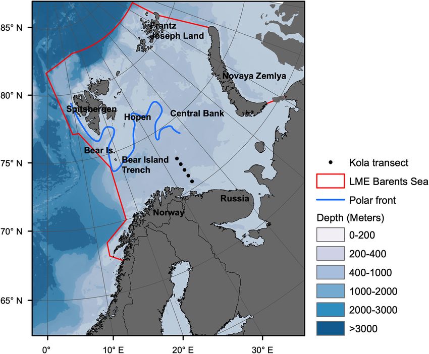
Pedersen et al.                                                                                                             Barents Sea Ecosystem Dynamics

Input Data to Ecopath Models                                               Balancing Ecopath Models
The Ecopath model for 1950 was based on an Ecopath model for               The BS ecosystem is a well-studied and ecological knowledge has
year 2000 but with biomass, fisheries, P/B and Q/B-values specific         accumulated. The Ecopath modeling allows us to evaluate the
for year 1950. Less information regarding many ecological groups           compatibility of the input data and identify uncertainty in the
was available for the period around 1950 and we chose year                 input data and in the model output because if the Ecopath model
2000 to represent a presumably similar year as 1950 with                   is unbalanced, the input data are not compatible. Before and
regard to temperature, and for balancing an annual average                 after balancing the Ecopath models, the pre-balance procedure
year 2000 Ecopath model. The average temperature in the                    (PREBAL) was used to check if input values were within accepted
Kola-section in 2000 was similar to 1950 (4.6◦ C vs. ca. 4.7◦ C)           ecological constraints (Link, 2010; Supplementary Appendix
(Dippner and Ottersen, 2001; Supplementary Figure 1). The                  4 Part D). Biomass, Q/B and P/B decreased with increasing
water temperature time-series from 1951 to 2013 (average from              TL, except for some mammals and bird groups that have
0 to 200 m depth, st. 3–7) from the Kola section (70◦ 300 N                high Q/B-values.
to 72◦ 300 N along 33◦ 300 E) [source: Knipovich Polar Research                Balancing the Ecopath models was done manually by checking
Institute of Marine Fisheries and Oceanography (PINRO)]1                   that EE ≤1 for the mammal, bird and fish groups where
(Figure 1) has been considered as a good indicator for the                 biomass input data were available. For groups where the biomass
temperature variability in the BS (Stige et al., 2010).                    was estimated by the Ecopath model from consumption by
   The annual average Ecopath model representing year                      its predators and catches, it was checked that biomass values
2000 was parameterized by the best available literature data               were within the range reported in the literature (Supplementary
(Supplementary Appendix 2). Data for biomass, catches, diet                Appendix 2). Gross efficiencies (P/Q) were checked to be
composition, production/biomass, consumption/biomass, and                  in accordance to the literature, and it was checked that
assimilation efficiency, were mainly derived from the BS. For              respiration/assimilation were

Pedersen et al.                                                                                                      Barents Sea Ecosystem Dynamics

Ecosim Time-Series Fitting, Model                                           combination of vulnerabilities gives the best statistical fit
Calibration, and Cross-Validation                                           using sums of squares (SS) and Akaike’s Information Criterion
                                                                            modified for small samples (AICc) as criteria to select the most
In fitting and calibrating ecological models, there is a potential
                                                                            parsimonious model (Akaike, 1974; Kletting and Glatting, 2009).
risk of overfitting models (Wenger and Olden, 2012). To evaluate
                                                                               The fitting and model evaluation procedure include several
Ecosim models, the model fit to time-series data, model behavior
                                                                            steps. (i) The sensitivities of SS for the chosen number of model
and the model’s ability to predict a part of the time-series not used
                                                                            vulnerabilities for each predator-prey interaction or predator
in the fitting (cross-validation) were considered. We performed a
                                                                            were calculated and FGs with the highest sensitivities were
cross-validation where the available time-series were split into a
                                                                            selected. (ii) It was searched iteratively for values of vulnerabilities
part (ca. 75%) used for model fitting (1950–1996) and a part used
                                                                            among the selected vulnerabilities to minimize the SS for the
for testing the predictability of the models (1997–2013) (Bergmeir
                                                                            period 1950–1996. (iii) Plots of model-fitted and observed time-
and Benítez, 2012; Wenger and Olden, 2012). A model’s ability
                                                                            series of biomasses and catches and SS for separate FG were
to predict for a time-period not used in fitting informs about
                                                                            visually inspected to evaluate model fit to observation data
its transferability. Transferability has been emphasized as an
                                                                            and assess if the model behavior was credible (Mackinson,
important aspect of model evaluation and cross-validation has
                                                                            2014; Heymans et al., 2016). To assess the effects of fisheries,
been suggested as a method to assess transferability and reduce
                                                                            environmental drivers and trophic factors (vulnerabilities),
risk of overfitting (Wenger and Olden, 2012).
                                                                            alternative models were tested. Alternative models were fitted
    Ecosim models were fitted to time-series for the period 1950–
                                                                            without fishery data (baseline models with no catch or fishing
1996 and calibrated by estimating predator-prey vulnerabilities
                                                                            mortality), with fisheries data and environmental forcing time-
(vij ). The number of vulnerabilities that can be estimated is
                                                                            series and with and without estimating vulnerabilities resulting in
equal to the number of independent time-series minus one (Scott
                                                                            a SS and an AICc-value per model. (iv) In the model prediction
et al., 2016). A common approach in Ecosim calibration/fitting to
                                                                            runs for the period 1997–2013, the predictability of models was
time-series has been to fit a spline-function which is considered
                                                                            assessed by calculating the SS for model output biomass and
a proxy for primary production, and then relate this spline
                                                                            catches and the corresponding observed data.
function to environmental proxies, such as NAO-indices and
                                                                               To assess the effect of climatically forced phytoplankton
water temperature (Skaret and Pitcher, 2016; Bentley et al.,
                                                                            primary production (PPR), in Ecosim, two alternative forcing
2017). However, we found it more appropriate to include a well-
                                                                            time-series were tested; a constant PPR-proxy and a PPR-
documented relationship for PPR as an environmental driver.
                                                                            proxy based on the relationship between phytoplankton primary
Before the Ecosim model was fitted to time-series, the time-series
                                                                            production and open-water area (Supplementary Appendix 4
were categorized into “forcing” (forcing the model to time-series
                                                                            Part A). A capelin larvae mortality proxy was calculated based
values), “absolute” (absolute values were used), “relative” (relative
                                                                            on the relationship between biomass of small herring and capelin
values, such as catch per unit effort were used). A total of 84 time-
                                                                            larvae mortality rate (Supplementary Appendix 4 Part A) and
series were used as input in the time-series fitting, including time-
                                                                            the proxy was used to force mortality rates of capelin (0–2)
series on absolute biomass (n = 32), relative biomass (n = 15),
                                                                            in model fitting.
forced biomass (n = 3), forced catch (n = 9), catches (n = 9),
                                                                               The possible effects of change in ice-coverage on ice-algae
fishing mortality (n = 14), harvesting effort (n = 2). This amounts
                                                                            primary production were tested by modifying model M10 by
to a total of 56 time-series on absolute and relative biomasses and
                                                                            forcing ice-algae biomass directly by the ice-cover in a model M11
catches that were used to calculate sum of squares and a potential
                                                                            run (Supplementary Appendix 4 Part A) for the period 1950–
maximum of 55 vulnerabilities could be fitted. A lognormal
                                                                            2013, and the results from model M11 were compared to model
error distribution was assumed minimizing the sum of squares
                                                                            M10 without forcing of the ice-algae. To test if the invasive red
of log observed values from log modeled values (Christensen
                                                                            king crab and the expanding snow crab may have affected the
et al., 2005). There were equal weights of each time-series, thus
                                                                            ecosystem, models with snow-crab and red king crab groups were
the absolute scale of time-series values did not influence the
                                                                            run for the period 2000–2013 (Supplementary Appendix 4 Part
sum of squares. The mesozooplankton biomass time-serie mainly
                                                                            E). The year 2000 model with 26 estimated vulnerabilities from
comprising the FGs medium sized copepods, large calanoids, and
                                                                            model M10 was run with (model M12) and without (model M13)
small copepods, was not used in the fitting but was compared to
                                                                            forcing by observed crab biomass time-series (Supplementary
the model output of the sum of biomass of its FGs. In addition,
                                                                            appendix 4 Part A), and the output biomasses from the Ecosim
various environmental time-series were used as driving forces for
                                                                            models were compared.
the model (Supplementary Appendix 4 Part A,B).
    An automatic step-wise fitting procedure was used to calibrate
the Ecosim-model to observed time-series for biomass fishing                Monte Carlo Simulations and Model
mortalities and catches (Scott et al., 2016). This procedure                Evaluation
statistically estimates how much fishery time-series, trophic               For model(s) considered to have most support assessed by the
interactions (predator-prey vulnerabilities) and environmental              stepwise fitting for the period 1950–1996, inspection of model
time-series contribute to model fit. The stepwise fitting procedure         behavior and test of predictability for the period 1997–2013,
constructs a series of model permutations with increasing                   Monte Carlos simulations (MCS) were run to assess uncertainty
number of estimated vulnerabilities (v) and determines which                in output values from Ecopath and Ecosim. In the MCS,

Frontiers in Marine Science | www.frontiersin.org                       6                                   September 2021 | Volume 8 | Article 732637
Pedersen et al.                                                                                                                        Barents Sea Ecosystem Dynamics

input values were randomly sampled from uniform distributions                                 on TL. The TLj of each predator group j was calculated using the
with the width of the distributions corresponding to pedigree-                                equation:
                                                                                                                              n
specified input uncertainty level for biomasses, P/B and Q/B                                                                X
values (Supplementary Appendices 1, 2), and the MCS routine                                                      TLj = 1 +       DCij TLi                  (6)
included 200 successful trials with balanced models. Each trial                                                                i=1

had up to 10,000 runs where Ecopath input parameter values                                    Where DCij is the proportion of prey i in the diet of predator j
were drawn and it was tested if the resulting Ecopath model was                               and TLi is the trophic level of group i. In Ecopath it is assumed
balanced. To evaluate uncertainty and compare model outputs                                   that all the detritus groups have trophic level 1.
with observed data, the 0.025 and 0.975 percentiles of the MCS                                   Trophic transfer efficiency calculated for a given trophic level
outputs were calculated.                                                                      is the ratio between the sum of exports plus the flow that is
   To evaluate the model fit, Taylor diagrams were used to                                    transferred from one trophic level to the next and the throughput
simultaneously visualize the correlation (Pearson) between                                    on the trophic level (Christensen and Walters, 2004).
observed and modeled time-series, the root-mean-square                                           The sum of all direct and indirect effects of a FG on the food
difference (RMS) and the ratio of the standard deviations of the                              web were quantified applying mixed trophic impacts (Heymans
simulated and the observed time-series (RSD) (Taylor, 2001).                                  et al., 2014). The mixed trophic impact mij of a group is the
                                                                                              product of all net impacts for all possible pathways that link
Ecosystem Indicators                                                                          groups i and j (Christensen and Pauly, 1992; Libralato et al.,
It has been advised to use a variety of indicators at the community                           2006). The total impact of each ecological group ei is calculated as
level to detect ecosystem impacts of fishing (Fulton et al., 2005).                                                           v
                                                                                                                              u n 2
                                                                                                                              uX
The indicators should include groups directly impacted by the
                                                                                                                         ei = t     mij                        (7)
fishery, charismatic groups with slow dynamics and response
                                                                                                                                j6=i
(e.g., mammals) and groups with fast dynamics and response
(e.g., zooplankton). We calculated several indicators to assess                               A modified variant of the Kempton diversity index (Kempton
effects of harvesting and the ecosystem states and changes during                             Q) has been developed and implemented in EwE to measure the
the time period 1950–2013 (Table 2).                                                          effects of fishing or climate on species in whole ecosystem models.
    The trophic levels of catches and ecosystem biomass may be                                Kempton Q express biomass diversity of groups with TL ≥3 and
affected by fisheries and have been used as indicator for ecosystem                           was expected to decrease with ecosystem degradation (Ainsworth
changes, with both expected to decrease in response to size-                                  and Pitcher, 2006; Steenbeek et al., 2018).
selective exploitation (Branch et al., 2010). Ecopath calculates                                  Production of each functional group over the modeled time
trophic level (TL) of the FGs, catches and various indices based                              period was calculated and total ecosystem production/biomass
                                                                                              ratio and P/B-ratio of non-primary producers FGs and of
                                                                                              harvested FGs were calculated. These P/B-ratios were expected
TABLE 2 | List of indicators at ecosystem and functional group level.                         to increase if high exploitation intensity decreases the proportion
                                                                                              of long-lived exploited FGs biomass to total ecosystem biomass.
Indicator name and units                               Type                  Level            The fishing mortality rate (F, year−1 ) for each exploited FG
Total biomass (g C   m−2 )                          Composite             Ecosystem           on a biomass basis (F = Y/B) was calculated as the ratio of
Total production (g C m−2 year−1 )                  Composite             Ecosystem           annual catch yield (Y, g C m−2 year−1 ) and biomass (g C
Total consumption (g C m−2 year−1 )                 Composite             Ecosystem           m−2 ). Fishing mortality is strongly positively related to fishing
Ecosystem production/biomass                        Composite             Ecosystem           effort. The ratio of annual catch yield to annual production
Kempton diversity index Q                           Composite             Ecosystem           (Y/P = catch yield/production) will be used an indicator for
Transfer efficiency (%)                              Trophic              Ecosystem           intensity of exploitation of exploited groups (Mertz and Myers,
Trophic level (TL)                                   Trophic             Funct. group         1998). The optimal FG specific exploitation rate (Y/P) that
Mixed trophic impacts of group (MT)                  Trophic             Funct. group         correspond to maximum sustainable yield from single stock
Total impact of group                                Trophic             Funct. group         considerations have been assessed to be about or slightly below
Ecosystem production/biomass of                       Fishery             Ecosystem           0.5, i.e., approximately equal fishing and natural mortality rate
harvested groups                                                                              (Patterson, 1992; Zhou et al., 2012).
Total catch                                           Fishery             Ecosystem
Trophic level of catch (TLc )                         Fishery             Ecosystem
Gross efficiency of fisheries (%)                     Fishery             Ecosystem           RESULTS
Catch as proportion of production                     Fishery            Funct. group
[Exploitation rate (Y/P) = annual                                                             Model Parametrization, Evaluation, and
catch/production]
Catch/Biomass ratio [Fishing mortality                Fishery            Funct. group
                                                                                              Fitting of Ecosim Models
(Y/B) = catch/biomass, year−1 ]                                                               Initially in the balancing procedure, production of pelagic fish
                                                                                              prey was less than consumption (i.e., EE > 1.0) in the year
Indicator type is categorized into; composite (expected to indicate both trophic and
fishery effects), trophic (expected to indicate trophic effects), and fishery (expected       2000 and 1950 models, and the biomass values for capelin
to indicate fishery effects).                                                                 and polar cod had to be increased relative to initial values

Frontiers in Marine Science | www.frontiersin.org                                         7                                  September 2021 | Volume 8 | Article 732637
Pedersen et al. Barents Sea Ecosystem Dynamics
(Supplementary Appendices 2, 4 Part F) to balance the models. minke whale, harp seals, Northeast Arctic cod (3+), coastal
In the balancing of the 1950-model, biomass values and total cod (2+), saithe (3+), and long rough dab (Hippoglossoides
mortality rates for the small herring, capelin and polar cod were platessoides) (Supplementary Table 1). For M8 with 51 estimated
increased relative to the initial values to balance the need for vulnerabilities, 29 vulnerabilities were >>2 (Supplementary
prey (Supplementary Appendix 4 Part F). Most FGs except for Table 2) and many estimated vulnerabilities were from trophic
the mammal and bird groups in the balanced year 2000 and interactions with lower trophic level groups without time-series
1950-models had relatively high EE’s indicating that most of for biomass or catch. Further results presented were based on the
the production from most groups were consumed by groups M10 model since it had the lowest prediction SS (Table 3).
within the model. For the model M10 forced by PPR-proxy and small-herring
All models fitted to time-series for the 1950–1996 time-period induced mortality on capelin larvae, modeled biomass time-
without estimated vulnerabilities (M1, M3, M5, M7, and M9) series for most high trophic level (TL > 3) groups [minke
had higher AICc and poorer fit than the corresponding models whales, harp seals, Northeast Arctic cod (3+) and saithe (3+)]
with estimated vulnerabilities (M2, M4, M6, M8, and M10) corresponded well with the observed time-series (Figure 2).
(Table 3). Among the former models, the baseline model M2 For haddock (3+), the modeled biomass was lower than the
fitted without fisheries data had much higher AICc than the observed biomass after ca. 2005 (Figure 2). Modeled (M10)
models (M4, M6, M8 and M10) fitted to fisheries data and with and observed time-series for the boreal fisheries-exploited FGs
estimated vulnerabilities (Table 3). The two models (M8 and Northeast Arctic cod (3+), minke whale, large redfish, large
M10) with estimated vulnerabilities and forced by the capelin Greenland halibut and saithe (3+), had relatively high (Spearman
(0–2) mortality proxy had lower AICc-values than models (M4 rs > 0.46) positive correlations with modeled values for the
and M6) fitted without the mortality proxy (Table 3). Model period 1950–2013. In contrast, harp seal and pelagic amphipods,
M10 forced by PPR-proxy and with 26 estimated vulnerabilities had negative correlations (Figure 3). Capelin groups and polar
had higher AICc than model M8 forced by constant PPR cod (2+) had moderate (rs from 0.40 to 0.65) positive correlations
with 51 estimated vulnerabilities. However, model M10 with 26 with modeled values, while polar cod (0–1) and haddock (3+)
vulnerability values had lower prediction SS (SS for the prediction had no or very low (rs from 0.0 to 0.06) correlation to modeled
period 1997–2013) than M8 which had far more (n = 51) values. The ratio of standard deviations showed that the observed
estimated vulnerabilities. Time-series of model biomasses from time-series of haddock (3+), Scyphozoa, pelagic amphipods and
exploited fish groups for models forced by the PPR-proxy had Thysanoessa had high temporal variability and were not highly
a more U-shaped trend during the period 1950–2013 than for correlated with the modeled values. Observed time-series of long
models forced by constant PPR. rough dab and northern shrimp (not shown in Figure 3) also had
For M10, all trophic interactions with estimated vulnerabilities relatively high temporal variability.
included at least one mammal or fish groups with time-series In the models (M1-M6) lacking mortality forcing on capelin
(Supplementary Table 1). Most (n = 18) of the 26 fitted (0–2), the capelin groups in the Ecosim model did not follow the
vulnerabilities were low (vulnerability values < 2) indicating large observed changes from the early 1980s onwards with a large
bottom-up effects, and the high vulnerabilities indicating top- decrease in biomass 1985 and later periodical ups and downs
down effects were estimated for interactions with top-predators; (Figure 2). For the polar cod groups, the modeled biomasses were
TABLE 3 | Overview of sum of squares for fit (1950–1996) and prediction (1997–2013) for alternative Ecosim models.
Model Name Fitting 1950–1996 Prediction 1997–2013
No Vs Total SS AICc Total SS SS non-fisheries
M1 Baseline 0 827 123 372 372
M2 Baseline 2 821 122 374 374
M3 Fishing + constant PPR 0 2,256 808 15,168 9,622
M4 Fishing + constant PPR 45 743 -233 547 421
M5 Fishing + PPR-proxy 0 17,880 2,932 77,290 48,427
M6 Fishing + PPR-proxy 35 756 –239 512 402
M7 Fishing + constant PPR + CapM-proxy 0 1,680 506 11,683 7,607
M8 Fishing + constant PPR + CapM-proxy 53 526 –568 352 288
M9 Fishing + PPR-proxy + CapM-proxy 0 17,441 2,907 73,987 46,536
M10 Fishing + PPR-proxy + CapM-proxy 26 640 –428 344 289
Models were fitted to time series for the period 1950–1996 for biomasses, fishing mortalities, fishing effort, and catches and estimating vulnerabilities (V) by the step-wise
fitting routine. Time-series for environmental drivers include a series with constant phytoplankton primary production (constant PPR), a series with phytoplankton primary
production driven by the ice-cover and open water area (PPR-proxy), and a capelin (0–2) mortality proxy (CapM-proxy). Sum of squares (SS) for the period 1997–2013
was calculated to test the prediction ability of the models fitted for the earlier period. Sum of squares shown in bold for baseline models are calculated for only non-fisheries
data and are not comparable to SS for model M3-M10 calculated for all data. SS, sum of squares calculated for model output and time-series observations; AICc, Akaike
Information criterion.
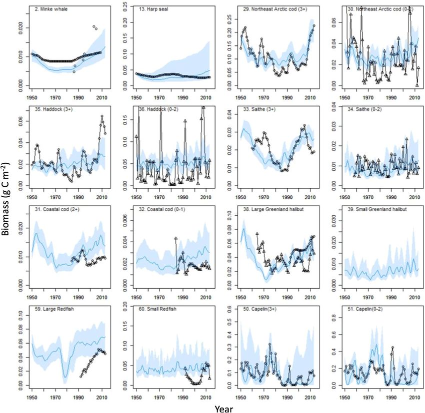
Frontiers in Marine Science | www.frontiersin.org 8 September 2021 | Volume 8 | Article 732637Pedersen et al. Barents Sea Ecosystem Dynamics FIGURE 2 | Biomass (g C m−2 ) changes for functional groups during 1950–2013 for modeled (model M10, continuous blue line) and observed (circles, absolute biomasses; triangles, relative biomasses). Blue line shows mean value and blue bands shows 2.5 and 97.5 percentiles from 200 Monte Carlo replicates. larger than the observed and the peaks in observed polar cod during the period 1990–2013, but the simulated biomass time- group biomasses around 2006 was not reproduced by the model series did not track the relative large year-to-year changes in the which predicted increases in biomass (Supplementary Figure 2). observed krill biomass indices (Supplementary Figure 2). The For northern shrimp, model M10 did not reproduce the peak Russian and Ecosystem survey time-series for krill biomass, were in observed biomass around 1980, but both model and observed moderately positively correlated for the time period (1980–2005) biomass had similar increasing trends after 1990 (Supplementary of overlapping measurements (Spearman rs = 0.39, P = 0.05). Figure 2). Biomasses of other pelagic lower trophic level groups, The modeled biomass for medium-sized copepods and large such as Thysanoessa and medium-sized copepods, had more calanoids had increasing trends after ca. 1995 contrasting the complex temporal variability. Both the modeled Thysanoessa relative stable biomass in the observed mesozooplankton biomass and the observed krill time-series showed an increasing trend time-series (Supplementary Figure 2). Modeled biomass trends Frontiers in Marine Science | www.frontiersin.org 9 September 2021 | Volume 8 | Article 732637
Pedersen et al.                                                                                                                      Barents Sea Ecosystem Dynamics

                                                                                        of snow and red king crab in the diet of predators, and the
                                                                                        importance of prey groups in the diet of the crab groups.
                                                                                        Increasing snow crab and red king crab biomass in model M13
                                                                                        led to a positive effect on predator biomass (e.g., Northeast
                                                                                        Arctic cod 3+) and negative effects for crab prey (Supplementary
                                                                                        Appendix 4 Part E).

                                                                                        Food Web Structure and Major Flow
                                                                                        Pathways
                                                                                        Trophic levels in the BS ecosystem ranged from 1 for primary
                                                                                        producers to 5.1 for Polar bear in the year 2000 and 1950 models
                                                                                        (Supplementary Appendix 4 Part F). Total biomass, production,
                                                                                        consumption and total system throughput were slightly (0.1–
                                                                                        11%) lower in the 2000 than in the 1950 model (Table 4). In the
                                                                                        year 2000 model, the total ecosystem biomass (13.7 g C m−2 )
                                                                                        was mainly comprised of biomass from detritivorous benthic
                                                                                        invertebrates (5.3 g C m−2 ), phytoplankton (2.0 g C m−2 ), other
                                                                                        herbivorous zooplankton (1.5 g C m−2 ) and krill (1.1 g C m−2 )
                                                                                        (Supplementary Table 4). Atlantic cod, the main fishery target,
                                                                                        had a biomass of 0.10 g C m−2 .
  FIGURE 3 | Taylor diagram showing correlation (Pearson r), residual mean
  square (RMS), and ratio of the standard deviations (scaled) of model simulated
                                                                                           The total ecosystem production was 167 g C m−2 yr−1 with
  (model M10) and observed time-series. Reference point where observed is               major contributions from the primary producers: phytoplankton
  equal to modeled values is shown by green square. Symbol labels; minke                (110 g C m−2 yr−1 ) and ice algae (5.3 g C m−2 yr−1 ). At
  whales (MW), harp seals (HS), Northeast Arctic cod 3+ (NA3), coastal cod 2+           trophic levels between 2 and 3, the main producers were the
  (NC2), saithe 3+ (SA3), haddock 3+ (HA3), large Greenland halibut (GH), large
                                                                                        aggregated compartments microzooplankton and HNAN (19.1 g
  redfish (RFL), capelin 3+ (CA3), capelin 0–2 (CA0), Polar cod 2+ (PC2), polar
  cod 0–1 (PC0), lumpfish (LF), pelagic amphipods (PA), Thysanoessa (TH), and           C m−2 yr−1 ), bacteria (16.1 g C m−2 yr−1 ), other herbivorous
  Scyphomedusae (SC). Groups with higher variability in observed than in                zooplankton (8.2 g C m−2 yr−1 ), krill (2.7 g C m−2 yr−1 ) and
  modeled time-series, such as haddock age 3+, Thysanoessa, pelagic
  amphipods, and Scyphomedusae are positioned close to zero scaled
  deviation ratio.
                                                                                        TABLE 4 | Overview of ecosystem metrics for the year 1950 and 2000- Ecopath
                                                                                        models.

                                                                                                                                 Model
during 1950–2015 for many lower trophic level (TL < 3)
groups, i.e., detritivorous polychaetes and large bivalves, showed                      Metrics                          1950            2000      Change between
                                                                                                                                                   2000 and 1950 in
a similar U-shaped trend as the PPR-proxy with a slight                                                                                            (%) of year 1950
dip in the cold period from 1960 to 1980 (Supplementary
Figure 2). The long-lived groups, such as large bivalves and large                      Net Primary production (g       110.7            115.5             4.4
                                                                                        C m−2 year−1 )
epibenthic suspension feeders had smoother biomass trajectories
                                                                                        Sum of all exports (g C         –0.67            –0.48          −28.4
and showed a more pronounced U-shape than groups with higher
                                                                                        m−2 year−1 )
P/B and shorter lifespan, such as detritivorous polychaetes.
                                                                                        Sum of all consumption (g       221.15           207.84          −6.0
   The comparison of models with (M11) and without (M10)                                C m−2 year−1 )
forcing of ice-algae biomass and production showed that                                 Sum of all flows to detritus     82.9             86.1             3.8
sympagic amphipods were strongly negatively affected by the                             (g C m−2 year−1 )
reduction in ice-coverage after year 2000 (Supplementary                                Sum of all respiratory flows    110.8            106.2           −4.2
Appendix 4 Part G). There were much smaller effects on other                            (g C m−2 year−1 )
groups that fed on ice-algae or ice-algae detritus, but noticeable                      Total system throughput (g      414.3            399.6           −3.5
positive effects of high ice-algae production in the cold 1960–                         C m−2 year−1 )

1980 period were found for biomasses of ringed and bearded                              Sum of all production (g C      167.5            167.3           −0.1
                                                                                        m−2 year−1 )
seals, little auk, and Brünnich’s guillemot. Effects of variable
                                                                                        Total biomass (excl.             15.4             13.7          −11.2
ice-algae production on polar-cod, pelagic amphipods and harp                           Detritus) (g C m−2 )
seals were small.                                                                       Total catch                     0.0779           0.069          −11.4
   The increase in red king crab and snow crab in the crab-                             Mean trophic level of catch      3.72             3.77             1.1
biomass-forced model M12 affected relatively few groups in                              (TLc )
the comparison to model M13 without crab-biomass forcing                                Gross efficiency (catch/net    0.00070       0.00060            −15.1
(Supplementary Appendix 4 Part E). The magnitude and                                    primary production)
direction of the effects were closely related to the importance                         Transfer efficiency (%)          19.5             18.0           −7.5

Frontiers in Marine Science | www.frontiersin.org                                  10                                      September 2021 | Volume 8 | Article 732637
Pedersen et al. Barents Sea Ecosystem Dynamics detritivorous benthic invertebrates (3.1 g C m−2 yr−1 ). At higher interactions and a connectance index of 0.095. The FGs with trophic levels (TL > 3), major producers were capelin (0.45 g C most groups (n) preying on them were; Thysanoessa (n = 43), m−2 yr−1 ), other planktivorous fishes (0.44 g C m−2 yr−1 ) and pelagic amphipods (n = 35), small herring (n = 33), medium sized shrimps (0.17 g C m−2 yr−1 ). Other demersal and benthic fish copepods (n = 31), capelin age 0–2 (n = 30), and northern shrimp had a production of 0.17 g C m−2 yr−1 ) and cod had a production (n = 29). of 0.08 g C m−2 yr−1 . Polar bear, whales, seals, cod, other The five FGs with highest total trophic impact (see Eq. 7) in demersal and benthic fishes, capelin and the zooplankton groups the year 2000 model were; (1) diatoms, (2) polar cod (2+), (3) had somewhat higher biomass, production and consumption in Thysanoessa, (4) medium sized copepods and (5) small benthic the 1950 that the 2000 model (Supplementary Figure 3). molluscs (Figure 5). These FGs had contrasting trophic impacts Four major pathways for carbon flow from lower to higher depending on their trophic position (Figure 5). Diatoms had trophic levels were evident for the year 2000 model (Figure 4); a positive impact as food source for many lower trophic level the microbial food web pathway, the copepod pathway, the krill FGs and had a much larger impact than autotrophic flagellates, pathway and the benthic invertebrate pathway. With regard to the other phytoplankton group (Figure 5). Medium sized the importance as prey, the krill compartment comprised of copepods and large calanoids had a positive impact as prey for the FGs Thysanossa and large krill had the most (n = 8) major planktivorous fishes and pelagic predatory groups (chaetognaths, prey flows (i.e., among the three largest flows to a predator cephalopods, Ctenophora, scyphomedusa, and northern shrimp). compartment from prey compartments) (Figure 4). Pelagic The krill groups also had a strong positive impact as prey for planktivorous fishes, herbivore zooplankton, and detritus had the demersal fishes, some bird groups and several whale and seal FGs second most connections with predator compartments with five (Figure 5). However, the krill groups also had negative impact major flows. Whereas, krill had major flows to five top-predator on some other planktonic invertebrate groups. Capelin and polar compartments, the herbivorous zooplankton compartments had cod had positive impacts as prey for demersal fish FGs, seals only one major flows to a top-predator compartment (Figure 4). and some whale groups, and negative impacts as predators on The diet matrix of the year 2000 -model including the snow- krill, the copepod groups and other pelagic zooplankton FGs crab and red king crab groups had a total of 1,029 feeding (Figure 5). Northeast Arctic cod (3+) had negative impacts as FIGURE 4 | Carbon flows between aggregated major compartments based on the Ecopath model for year 2000 with four major pathways for carbon flows from lower to higher trophic levels. (i) the microbial food-web pathway (violet lines), (ii) the copepod pathway (yellow lines), (iii) the krill pathway (red lines), and (iv) the benthic invertebrate pathway (brown lines). Functional group outputs are aggregated according to Table 1. Thick lines shows major flows, i.e., among the three largest flows to each aggregated compartment. Thin lines shows smaller flows. “H” in circles indicate harvested compartments. Frontiers in Marine Science | www.frontiersin.org 11 September 2021 | Volume 8 | Article 732637
Pedersen et al.                                                                                                                  Barents Sea Ecosystem Dynamics

  FIGURE 5 | Mixed trophic impact for the year 2000-model. Mixed trophic impacts are shown from the 30 ranked functional groups with highest total impact (column
  names) on 50 selected impacted functional groups (rows).

predator on several other fish FGs and positive impact as prey for                   Berdnikov et al. (2019) and lower (–0.21 and –0.25) than the TL’s
Greenland shark and dolphins (Figure 5). Northeast Arctic cod                        from Blanchard et al. (2002) and Bentley et al. (2017).
also had negative effects on seal and fish FGs that shared prey
with cod (Figure 5).
   Trophic levels estimated by our Ecopath model for year
                                                                                     Temporal Variation in Ecosystem
2000 differed considerably from previously published TL-values                       Properties and Effects of Exploitation
from mass-balance models for the BS (Supplementary Table 3).                         and Climate Variability
TL-values from our model were on average higher (0.14 and                            The total catch in the BS peaked in the late 1970s mainly driven
0.25) than the trophic levels from Dommasnes et al. (2002) and                       by the large catches of capelin (Supplementary Figure 5). The

Frontiers in Marine Science | www.frontiersin.org                               12                                     September 2021 | Volume 8 | Article 732637
Pedersen et al. Barents Sea Ecosystem Dynamics
FIGURE 6 | Overview of changes in ecosystem indicators from Ecosim model M10 with Monte Carlo simulations. (A) Trophic level of catch, (B) Kempton’s diversity
index Q, (C) total system production/biomass ratio of non-primary producer functional groups, (D) production/biomass ratio based on sum of production and sum of
biomass of harvested functional groups. Blue line shows mean value and blue bands shows 2.5 and 97.5 percentiles from 200 Monte Carlo replicates.
catches of mammals decreased during the 1950s and 1960s, The Kempton’s diversity index Q changed moderately during
stabilized during 1965–1990 and decreased to low levels after 1950–2015 but had lower values at the end of the time-period
2005 (Supplementary Figure 5). Catches of cod had a decreasing than in the beginning (Figure 6). Ecosystem P/B for non-primary
trend from the 1950s and reached a minimum in the period producing FGs showed a modest increase in the 1970–1980s, but
from 1980 to 1990 and then increased to 2013. Other demersal there was a clear peak in P/B for harvested FGs in the 1970–1980s.
fishes had a peak in the 1970s due to large catches of redfish Trophic level of the catch (TLc) decreased from 1950 to 1985
and Greenland halibut, and had an increase after year 2000 followed by three periods of ups- and downs corresponding to
(Supplementary Figures 5, 6). periods of opening and closure of the capelin fishery (Figure 6).
The trend in the PPR-proxy showed an U-shaped trend Patterns over time for catches and fishing mortalities (F = Y/B)
with low values in the 1960–1980s (Supplementary Figure 1). varied substantially between FGs and for Polar bear, minke-
Similar U-shaped biomass trends were evident for mammal and whale, harp seals and small herring, catches and catch as
birds, total fish biomass, demersal fishes, pelagic invertebrate, proportion of production (Y/P) showed decreasing trends after
and benthic invertebrates group (Supplementary Figure 4). 1950 (Figure 7 and Supplementary Figures 6, 7). For large
Total biomass of the ecosystem decreased from 1950 to the Greenland halibut, large redfish, polar cod (2+), northern shrimp
lowest values around 1970 and thereafter increased toward and capelin (3+), catches and (Y/P) rose rapidly during the 1970s
2013 (Supplementary Figure 4). In contrast to biomass trends followed by decreasing trends. Catches of the large gadoids; the
of most other groups, pelagic fish biomass was highest in Northeast Arctic and coastal cod groups, haddock and saithe,
the period 1970–1980 largely driven by the high capelin showed temporal variability with low catches in the 1980’s. Y/P
biomass at this time. for these FGs peaked in the period 1970–1980 and were relatively
Frontiers in Marine Science | www.frontiersin.org 13 September 2021 | Volume 8 | Article 732637Pedersen et al. Barents Sea Ecosystem Dynamics
FIGURE 7 | Changes in ratio of catch to production (Y/P) of exploited Ecopath groups during the period 1950–2013. Based on data from M10 Ecosim model. Blue
line shows mean value and blue bands shows 2.5 and 97.5 percentiles from Monte Carlo replicates.
low after 1980 (Figure 7). Y/P were above 0.5 in periods for all due to reduced ice-coverage and larger open water area had a
exploited FGs except for Northern shrimp and Polar cod (2+) positive impact on production and biomass of boreal FGs at
that had low fishing mortalities and low Y/P’s (Figure 7 and all trophic levels.
Supplementary Figure 7).
Model Evaluation and Fitting to
Time-Series
DISCUSSION The Ecopath models initial values for biomass and production
of capelin and polar cod in year 2000 and 1950 did not match
Main Findings the consumption demand from predators and biomasses had to
Intense harvesting had clear negative effects on the biomasses be increased to match the consumption demand. This could be
of exploited and long-lived high trophic level FGs, such as due to underestimation of capelin and polar cod stocks as shown
mammals, large gadoids, Greenland halibut and redfish. Decrease in previous studies (Gjøsæter et al., 1998; Hop and Gjøsæter,
in fishing pressure the later years contributed to increases of 2013). An alternative explanation for the apparent production-
biomasses for many higher trophic level FGs, indicating a consumption mismatch may be that the consumption on
recovery period. An increase in primary production after ca. 1990 planktivorous fish has been overestimated due to bias in the diet
Frontiers in Marine Science | www.frontiersin.org 14 September 2021 | Volume 8 | Article 732637Pedersen et al. Barents Sea Ecosystem Dynamics
composition of predators. Diet data for most predators except the Ecosim models react to perturbations and such effects should
for Northeast Arctic cod were not adjusted for possible prey- be further investigated.
group-specific differences in digestion rates. Since large fish prey
are more slowly digested than smaller prey (Salvanes et al.,
1995), predator diet proportions of pelagic fishes may have been Ecosystem Structure and Major Carbon
overestimated relative to smaller invertebrate prey. Flow Pathways and Compartments
The cross-validation procedure revealed that the model (M8) The four dominant carbon flows pathways (microbial food
with fisheries and capelin mortality proxy and constant primary web, copepod, krill, and benthic invertebrate pathways) differed
production had a better fit and lower AICc for the fitting period regarding P/B of their contributing FGs and their functions
but higher sum of squares for the prediction period than for the as prey sources. The carbon flows within the microbial food
model M10 with ice-coverage forced primary production. This web with high P/B and high turnover merges with the krill
led to the conclusion that M10 was the model with most support and copepod pathway and “hitch-hikes” to higher trophic levels.
and this model showed an effect of increasing PPR especially in Microzooplankton made up large proportions (10–32%) of the
the last part of the period 1950–2013. diets of medium zooplankton, large calanoids, small copepods
The moderate effects of including snow crab and red king crab and Thysanoessa in the model, which is consistent with previous
FGs in the year 2000 model run with forced biomasses of red king studies suggesting a substantial flow from the microbial food web
crab and snow crab from year 2000 to 2013 suggest that these to higher trophic level pelagic FGs in the BS (Hansen et al., 1996;
FGs were unlikely to have a major effect at the whole ecosystem De Laender et al., 2010).
level during the studied time-period. For red king crab which The importance of the copepod pathway was indicated by
has a coastal distribution in the southern part of the BS, strong the high total impact ranks of medium sized copepods and
effects on local and regional scale on the bottom fauna have been large calanoid copepods, mainly resulting from impacts as prey
described (Oug et al., 2011), and similar effects may be expected for planktivorous fish FGs and pelagic carnivorous invertebrate
following ongoing the snow crab expansion. FGs, but also impacts as consumers of microzooplankton and
phytoplankton. Copepods are also major prey for early fish
stages. In contrast to the krill pathway, the copepod pathway
Comparison With Other Studies had less direct impact as prey for birds and mammals except
There was a good correspondence between trophic levels as prey for little auks and bowhead whales (Supplementary
estimated for 83 FGs in the Ecopath model for year 2000 and for Appendix 4 Part C).
independent data on trophic levels and δ15 N from stable isotope The krill pathway contributed to an energy-efficient carbon
data from the BS (Pedersen in prep.). The differences between flow to higher trophic levels and top-predators as seen in other
trophic levels estimated by our and other mass-balance models ecosystems (Murphy et al., 2007; Ruzicka et al., 2012). The
for the BS may be due to between-model differences in group fact that the krill groups were important as prey, but also as a
structure and diets of dominant FGs. predator and potential competitor for other zooplankton FGs,
Values for biomass, production and consumption of seals, suggest that krill may have a wasp-waist function in the BS
krill, mesozooplankton, and bacteria differ substantially between food web. The increase in biomass of krill and corresponding
our model and those published earlier for the BS (Supplementary increase in proportion of krill in the diet of age 1–2 year cod
Table 4). The twice as high food consumption from seals in after 1984 (Bogstad et al., 2015), suggest increased importance
our model compared to values given by Sakshaug et al. (1994), of krill during the last part of the time period. Advection of
was mainly due to lower Q/B-values used by Sakshaug et al. krill from the Norwegian Sea to the BS was found to be more
(1994). Further, production from krill in our year 2000 Ecopath prominent in warm years (Orlova et al., 2015), and is likely to
model was about twice that given by Sakshaug et al. (1994). have contributed to the increased importance of krill in the BS
For both krill groups, we used a higher P/B than Sakshaug during the warming period.
et al. (1994) (2.5 vs. 1.5 yr−1 ). Production by bacteria in our The detritus-based benthic invertebrate pathway transports
model was less than 25% of the value given by Sakshaug carbon to predatory benthos FGs, demersal and benthic fish
et al. (1994) and both Sakshaug et al. (1994) and Berdnikov and also some birds and mammals FGs. Field-based production
et al. (2019) used much higher P/B-values for bacteria (125–200 estimates for macrobenthos for the BS are scarce and uncertain,
year−1 ) than in our model (21.2 year−1 ). The P/B values for but local estimates of production range from 0.1 to 20 g C
the mesozooplankton, benthic invertebrate and meiofauna FGs m−2 year−1 (K˛edra et al., 2013, 2017). Despite the uncertainty,
in our model were much lower than the values from Blanchard P/B’s (You can also read