Numerical tools to study hydrogen flame acceleration
←
→
Page content transcription
If your browser does not render page correctly, please read the page content below
Numerical tools to study hydrogen flame acceleration
                              WCCM ECCOMAS Congress 2021

                                           January 11-15, 2021

                                              Luc Lecointre
                Sergey Kudriakov1 , Etienne Studer1 , Ronan Vicquelin2 , Christian Tenaud3

1    Université Paris Saclay, CEA, Service de Thermo-hydraulique et de mécanique des fluides, 91191, Gif
                                              sur Yvette, France
    2 Université Paris Saclay, CNRS, CentraleSupélec, Laboratoire EM2C, 91190, Gif-sur-Yvette, France
                        3 Université Paris Saclay, CNRS, LIMSI, 91400, Orsay, France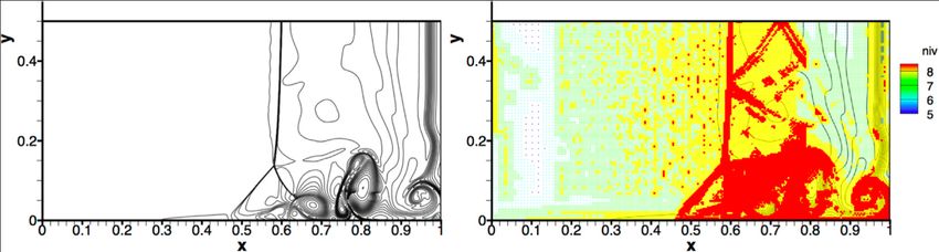
Introduction
Introduction

Introduction

 Inflammable gas dynamics in confined environment
    • Storage of flammable gas
    • Release of hydrogen in core reactor during nuclear accident

 Dynamic behaviour of the flame
    • Flame acceleration
    • Transition to Detonation
    • Influence of concentration gradients 1 , geometrical
      configuration...

 Experimental Setup 2

                                                                         Figure 1 – Shadowgraph sequence
                                                                         of DDT inside obstacle with
                                                                         vertical concentration gradient1

1. Boeck et al., Shock Waves (2016).
2. Scarpa et al., International Journal of Hydrogen Energy (2019).
              Luc Lecointre                          WCCM ECCOMAS 2021                    January 11-15, 2021   2 / 14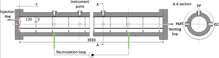
Introduction

Flame acceleration and transition to detonation

         Ignition               Laminar Flame

Flame acceleration phenomena

         Luc Lecointre          WCCM ECCOMAS 2021   January 11-15, 2021   3 / 14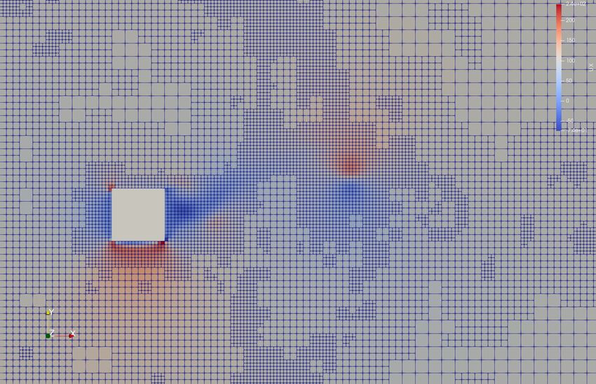
Introduction

Flame acceleration and transition to detonation

                                                                                    Wrinkled
         Ignition                          Laminar Flame
                                                               Thermo-diffusive   laminar flame
                                                                  instability

Flame acceleration phenomena

  • Thermodiffusive instabilities (Le < 1 flame
    wrinkling)

         Luc Lecointre                     WCCM ECCOMAS 2021                         January 11-15, 2021   3 / 14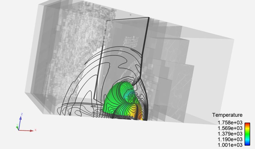
Introduction

Flame acceleration and transition to detonation

                                                                                      Wrinkled
         Ignition                          Laminar Flame
                                                               Thermo-diffusive     laminar flame
                                                                  instability
                                                                                               Turbulence
                                                                                             generation and
                                                                                               interaction
                                                                                               with flame

                                                                                  Slow Deflagration

Flame acceleration phenomena

  • Thermodiffusive instabilities (Le < 1 flame
    wrinkling)
  • Turbulence generation

         Luc Lecointre                     WCCM ECCOMAS 2021                           January 11-15, 2021    3 / 14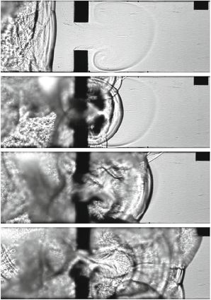
Introduction

Flame acceleration and transition to detonation

                                                                                       Wrinkled
         Ignition                          Laminar Flame
                                                               Thermo-diffusive      laminar flame
                                                                  instability
                                                                                                Turbulence
                                                                                              generation and
                                                                                                interaction
                                                                Shock formation                 with flame
                                                                 and interaction
                                                                   with flame
                                          Fast Deflagration                        Slow Deflagration

Flame acceleration phenomena

  • Thermodiffusive instabilities (Le < 1 flame
    wrinkling)
  • Turbulence generation
  • Shock interaction : Richtmyer Meshkov
    instability

         Luc Lecointre                     WCCM ECCOMAS 2021                            January 11-15, 2021    3 / 14
Introduction

Flame acceleration and transition to detonation

                                                                                              Wrinkled
         Ignition                                 Laminar Flame
                                                                      Thermo-diffusive      laminar flame
                                                                         instability
                                                                                                       Turbulence
                                                                                                     generation and
                                                                                                       interaction
                         Critical conditions ;                         Shock formation                 with flame
                            Transition to                               and interaction
                              detonation                                  with flame
       Detonation                                Fast Deflagration                        Slow Deflagration

Flame acceleration phenomena

  • Thermodiffusive instabilities (Le < 1 flame
    wrinkling)
  • Turbulence generation
  • Shock interaction : Richtmyer Meshkov
    instability

         Luc Lecointre                            WCCM ECCOMAS 2021                            January 11-15, 2021    3 / 14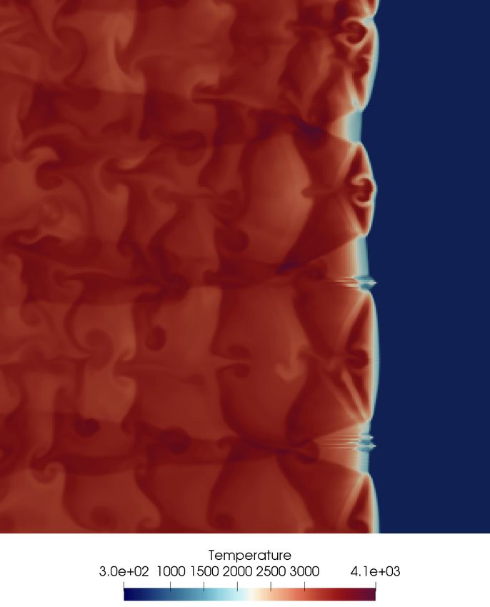
Introduction

Flame acceleration and transition to detonation

                                                                                              Wrinkled
         Ignition                                 Laminar Flame
                                                                      Thermo-diffusive      laminar flame
                                                                         instability
                                                                                                       Turbulence
                                                                                                     generation and
                                                                                                       interaction
                         Critical conditions ;                         Shock formation                 with flame
                            Transition to                               and interaction
                              detonation                                  with flame
       Detonation                                Fast Deflagration                        Slow Deflagration

Flame acceleration phenomena

  • Thermodiffusive instabilities (Le < 1 flame
    wrinkling)
  • Turbulence generation
  • Shock interaction : Richtmyer Meshkov
    instability
  • Impact of geometrical configuration : turbulent
    vortex, local hot spots...

         Luc Lecointre                            WCCM ECCOMAS 2021                            January 11-15, 2021    3 / 14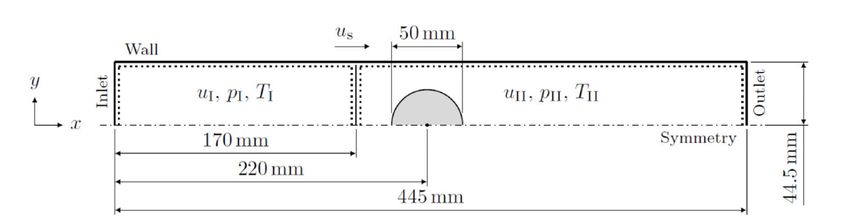
Introduction

Numerical tools/MR_CHORUS solver

 Navier-Stokes equation
                    wt + ∇ · (FE (w) − FV (w, ∇w)) = S(w), with w = (ρY1 , ..., ρYns , ρu, ρE )T                 (1)

 Numerical challenges 3
    • Multiscales in time and space
    • Compressible effects
    • Non callorically perfect gas

3. Tenaud, Roussel et Bentaleb, Computers & Fluids (2015).
             Luc Lecointre                         WCCM ECCOMAS 2021                       January 11-15, 2021   4 / 14
Introduction
Numerical tools/MR_CHORUS solver
Navier-Stokes equation
wt + ∇ · (FE (w) − FV (w, ∇w)) = S(w), with w = (ρY1 , ..., ρYns , ρu, ρE )T (1)
Numerical challenges 3
• Multiscales in time and space ⇒ Splitting operators with adapted solver
• Compressible effects
• Non callorically perfect gas
3. Tenaud, Roussel et Bentaleb, Computers & Fluids (2015).
Luc Lecointre WCCM ECCOMAS 2021 January 11-15, 2021 4 / 14Introduction
Numerical tools/MR_CHORUS solver
Navier-Stokes equation
wt + ∇ · (FE (w) − FV (w, ∇w)) = S(w), with w = (ρY1 , ..., ρYns , ρu, ρE )T (1)
Numerical challenges 3
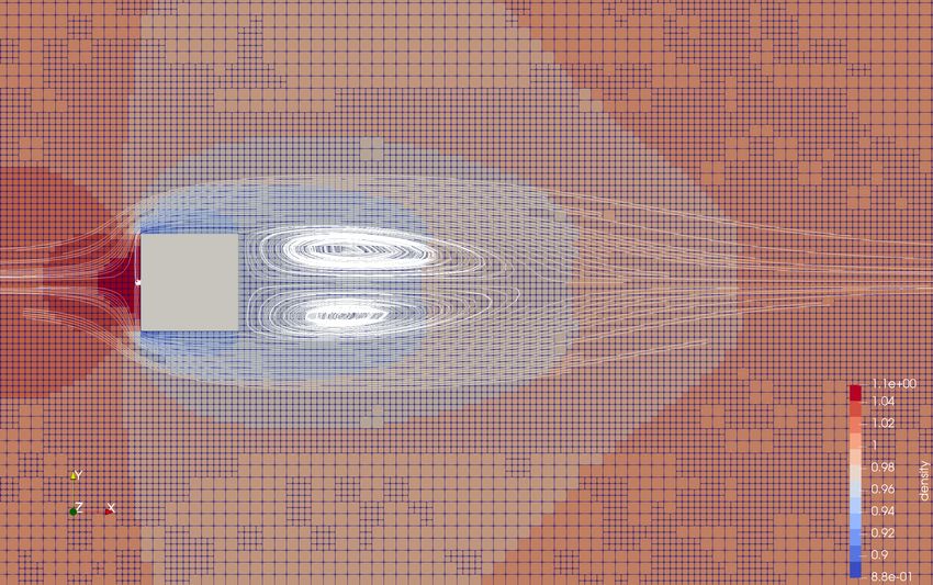
• Multiscales in time and space ⇒ Splitting operators with adapted solver / Adaptive refinement
• Compressible effects
• Non callorically perfect gas
Figure 2 – Multiresolution approach with dynamic graded Tree
3. Tenaud, Roussel et Bentaleb, Computers & Fluids (2015).
Luc Lecointre WCCM ECCOMAS 2021 January 11-15, 2021 4 / 14Introduction
Numerical tools/MR_CHORUS solver
Navier-Stokes equation
wt + ∇ · (FE (w) − FV (w, ∇w)) = S(w), with w = (ρY1 , ..., ρYns , ρu, ρE )T (1)
Numerical challenges 3
• Multiscales in time and space ⇒ Splitting operators with adapted solver / Adaptive refinement
• Compressible effects ⇒ Riemann approximate solver with flux limiter (OSMP scheme)
• Non callorically perfect gas
Figure 2 – Shock/boundary layer interaction. Isocontour of density and refined grid
3. Tenaud, Roussel et Bentaleb, Computers & Fluids (2015).
Luc Lecointre WCCM ECCOMAS 2021 January 11-15, 2021 4 / 14Introduction
Numerical tools/MR_CHORUS solver
Navier-Stokes equation
wt + ∇ · (FE (w) − FV (w, ∇w)) = S(w), with w = (ρY1 , ..., ρYns , ρu, ρE )T (1)
Numerical challenges 3
• Multiscales in time and space ⇒ Splitting operators with adapted solver / Adaptive refinement
• Compressible effects ⇒ Riemann approximate solver with flux limiter (OSMP scheme)
• Non callorically perfect gas ⇒ Extension of the Roe solver to realistic thermodynamic models
Figure 2 – Dependence of heat capacities on temperature with NASA polynomials
3. Tenaud, Roussel et Bentaleb, Computers & Fluids (2015).
Luc Lecointre WCCM ECCOMAS 2021 January 11-15, 2021 4 / 14OSMP scheme
OSMP scheme

Roe Approximate Riemann Solver

 Roe Solver 4                                                                         t
                                                                                    w2      w2
 Roe’s approach replace the Jacobian matrix evaluated at the                                       w3
 intersection A(w) = ∂FE (w)/∂w by a constant Jacobian matrix
 evaluated at the Roe average state w combination of left wL and
                                                                          w1 = wL                   w4 = wR
 right states wR
                        A(w) = A(wL , wR )                    (2)                                               x

4. Roe, Journal of Computational Physics (1981).
             Luc Lecointre                            WCCM ECCOMAS 2021                   January 11-15, 2021       5 / 14
OSMP scheme
Roe Approximate Riemann Solver
Roe Solver 4 t
w2 w2
Roe’s approach replace the Jacobian matrix evaluated at the w3
intersection A(w) = ∂FE (w)/∂w by a constant Jacobian matrix
evaluated at the Roe average state w combination of left wL and
w1 = wL w4 = wR
right states wR
A(w) = A(wL , wR ) (2) x
With non ideal gases
A(w) = A(ρ, Y 1 , ..., Y ns , u, h, χ1 , ...χns , κ) (3)
with compressibility factors
∂p ∂p
χi = and κ= (4)
∂ρi ˜,ρk,k6=i ∂˜
ρk
4. Roe, Journal of Computational Physics (1981).
Luc Lecointre WCCM ECCOMAS 2021 January 11-15, 2021 5 / 14OSMP scheme
Roe Approximate Riemann Solver
Roe Solver 4 t
w2 w2
Roe’s approach replace the Jacobian matrix evaluated at the w3
intersection A(w) = ∂FE (w)/∂w by a constant Jacobian matrix
evaluated at the Roe average state w combination of left wL and
w1 = wL w4 = wR
right states wR
A(w) = A(wL , wR ) (2) x
With non ideal gases
A(w) = A(ρ, Y 1 , ..., Y ns , u, h, χ1 , ...χns , κ) (3)
with compressibility factors
∂p ∂p
χi = and κ= (4)
∂ρi ˜,ρk,k6=i ∂˜
ρk
Flux expression
m
1 1X
FRoe1 = (FL + FR ) − δζ i |λi |r(i) (5)
i+ 2 2 2 i=1
with λi , r(i) and ζ i eigenvalues, eigenvectors and Riemann invariants of A(w)
4. Roe, Journal of Computational Physics (1981).
Luc Lecointre WCCM ECCOMAS 2021 January 11-15, 2021 5 / 14OSMP scheme
Roe Average state A(w) = A(ρ, Y 1 , ..., Y ns , u, h, χ1 , ...χns , κ)
Rule for the construction of the Roe Average State
A(w)(wL − wR ) = F(wL ) − F(wR ) (6)
5. Vinokur et Montagné, Journal of Computational Physics (1990).
Luc Lecointre WCCM ECCOMAS 2021 January 11-15, 2021 6 / 14OSMP scheme
Roe Average state A(w) = A(ρ, Y 1 , ..., Y ns , u, h, χ1 , ...χns , κ)
Rule for the construction of the Roe Average State
A(w)(wL − wR ) = F(wL ) − F(wR ) (6)
Roe average operator for primitive/conservatives variables √
ρL
{ρ, Yk , u, h} ⇒ (·) = θ(·)L + (1 − θ)(·)R with θ= √ √ (7)
ρL + ρR
Treatment of the compressibility factors χi and κ
A(w)(wL − wR ) = F(wL ) − F(wR )
ns
X
+ ⇒ ∆p = χi ∆ρi + κ∆˜
(8)
Roe average operator
i=0
Approximation of the compressibility factors with method of Vinokur and Montagné 5 :
Z 1 Z 1
κ̂ = κ[ρ(t), ˜(t)]dt χ̂i = χi [ρ(t), ˜(t)]dt (9)
0 0
Orthogonal projection on the ns − 1 dimension hyperplane defined by (8)
κ = P(κ̂) χi = P(χ̂i ) (10)
5. Vinokur et Montagné, Journal of Computational Physics (1990).
Luc Lecointre WCCM ECCOMAS 2021 January 11-15, 2021 6 / 14OSMP scheme
High order extension with OSMP scheme
One step monotonocity preserving (OSMP) scheme 6
New system of advection equations
∂ζ i ∂ζ
+ λi i = 0 with Λ = (u, ..., u, u − c s , u + c s )T (11)
∂t ∂x
6. V.Daru et Tenaud, Journal of Computational Physics (2004).
Luc Lecointre WCCM ECCOMAS 2021 January 11-15, 2021 7 / 14OSMP scheme
High order extension with OSMP scheme
One step monotonocity preserving (OSMP) scheme 6
New system of advection equations
∂ζ i ∂ζ
+ λi i = 0 with Λ = (u, ..., u, u − c s , u + c s )T (11)
∂t ∂x
Increase order in time and space with Lax-Wendroff procedure
1X o
Foj+1/2 = FRoe
j+1/2 + (Φ r)k,j+1/2 (12)
2 k
Flux limiter : Monotonicity preserving scheme (TVD scheme with improvement near extrema)
Φo−MP = max(Φmin , min(Φo , Φmax )) (13)
Riemann invariants recombination
Recomposition of the equations (11) with the same eigenvector u to improve flux limiter and keep relation
between variation of mass fraction and variation of mass energy
ns
bis X χ ∆P
ζ1 = ζ i E c − i = ∆(ρE ) + E c ∆ρ − H 2 (14)
i=1
κ c
6. V.Daru et Tenaud, Journal of Computational Physics (2004).
Luc Lecointre WCCM ECCOMAS 2021 January 11-15, 2021 7 / 14Numerical experiments
Numerical experiments

Realistic Thermodynamic model : Sod shock tube problem

                                                                                  0 ≤ x ≤ 25        25 < x ≤ 50
Properties
                                                                     P (bar)      1                 0.1
  • Sod shock tube with R22 gas, 640 cells and                       ρ(kg/m3 )    1                 0.125
    OSMP scheme of 7th order                                         N2 (%)       75.55             23.16
                                                                     R22 (%)      23.16             75.55
  • Species data with thermodynamic NASA
                                                                     O2 (%)       1.29              1.29
    polynomials
                                                                     γ            1.38              1.32

                                                                            Table 1 – initial conditions

                             Figure 3 – Density, velocity and temperature profiles at t = 20ms

             Luc Lecointre                            WCCM ECCOMAS 2021                          January 11-15, 2021   8 / 14
Numerical experiments
Realistic Thermodynamic model : Sod shock tube problem
0 ≤ x ≤ 25 25 < x ≤ 50
Properties
P (bar) 1 0.1
• Sod shock tube with R22 gas, 640 cells and ρ(kg/m3 ) 1 0.125
OSMP scheme of 7th order N2 (%) 75.55 23.16
R22 (%) 23.16 75.55
• Species data with thermodynamic NASA
O2 (%) 1.29 1.29
polynomials
γ 1.38 1.32
Table 1 – initial conditions
Figure 3 – Density, velocity and temperature profiles at t = 20ms
Luc Lecointre WCCM ECCOMAS 2021 January 11-15, 2021 8 / 14Numerical experiments
Realistic Thermodynamic model : Sod shock tube problem
0 ≤ x ≤ 25 25 < x ≤ 50
Properties
P (bar) 1 0.1
• Sod shock tube with R22 gas, 640 cells and ρ(kg/m3 ) 1 0.125
OSMP scheme of 7th order N2 (%) 75.55 23.16
R22 (%) 23.16 75.55
• Species data with thermodynamic NASA
O2 (%) 1.29 1.29
polynomials
γ 1.38 1.32
• OSMP adapted with combination of Riemann
invariants (14) Table 1 – initial conditions
Figure 3 – Density, velocity and temperature profiles at t = 20ms
Luc Lecointre WCCM ECCOMAS 2021 January 11-15, 2021 8 / 14Numerical experiments
Hydrodynamic instability : shock/bubble interaction
Parameters
pII = 1Bar ,
TII = 351.82K ,
Ms = 1.22
OSMP 7th order
Results
Figure 4 – Mesh and density gradient at τ = taII ,R22 /d0 = 1.15 for 256 cells in initial bubble diameter
Capture of Richtmyer–Meshkov instability with high order simulation
Luc Lecointre WCCM ECCOMAS 2021 January 11-15, 2021 9 / 14Numerical experiments
Reactive mixture : Detonation front
1D ZND structure
Respect stability criterion (heat release, induction length, overdriven velocity...) 7
Unstable case
Figure 5 – Oscillation of post-shock pressure for increasing induction length until quenching
7. Ng et al., Combustion Theory and Modelling (2005).
Luc Lecointre WCCM ECCOMAS 2021 January 11-15, 2021 10 / 14Numerical experiments
Reactive mixture : Acceleration of flame
Detonation initiation by reflected shock
T = 300K
Wall
• Two-steps chemistry flame P = 1atm
M = 2.5 Φ=1
• NASA poynomials
Luc Lecointre WCCM ECCOMAS 2021 January 11-15, 2021 11 / 14Numerical experiments
Reactive mixture : Acceleration of flame
Detonation initiation by reflected shock
T = 300K
Wall
• Two-steps chemistry flame P = 1atm
M = 2.5 Φ=1
• NASA poynomials
Luc Lecointre WCCM ECCOMAS 2021 January 11-15, 2021 11 / 14Numerical experiments
Reactive mixture : 2D Detonation
Detonation structure
2D Detonation front
• Detonation cell
• Shear layer
• Chemical induction layer
Luc Lecointre WCCM ECCOMAS 2021 January 11-15, 2021 12 / 14Numerical experiments
Reactive mixture : 2D Detonation
Detonation structure
Carbuncle instability
• Insufficient cross-flow dissipation
• Specific to Complete Riemann solver
• Amplified phenomena with heat release
Luc Lecointre WCCM ECCOMAS 2021 January 11-15, 2021 12 / 14Numerical experiments
Cure the carbuncle instabilities
Rotated solver 8
2
Rotational invariant property of Euler equation
X
n= αk nk
k=1
(ŵk )t + (f E (ŵk ))x̂ = 0 (15) n2
with ŵk = Tk wk and Tk rotation matrix
n
2
" N
#
1 1 X X
FRoe1 = (FL + FR ) − |αm
i+1/2 | δζ i |λi |r(i) (16)
i+ 2 2 2 m=1 i=1
n1
Figure 6 – Application of rotated solver
8. Ren, Computers & Fluids (2003).
Luc Lecointre WCCM ECCOMAS 2021 January 11-15, 2021 13 / 14Numerical experiments
Cure the carbuncle instabilities
Rotated solver 8
2
Rotational invariant property of Euler equation
X
n= αk nk
k=1
(ŵk )t + (f E (ŵk ))x̂ = 0 (15) n2
with ŵk = Tk wk and Tk rotation matrix
n
2
" N
#
1 1 X X
FRoe1 = (FL + FR ) − |αm
i+1/2 | δζ i |λi |r(i) (16)
i+ 2 2 2 m=1 i=1
n1
Figure 6 – Application of rotated solver
Not a high-order recomposition for now (diffusive solution)
8. Ren, Computers & Fluids (2003).
Luc Lecointre WCCM ECCOMAS 2021 January 11-15, 2021 13 / 14Conclusion
Conclusion

Conclusion

Objective : complete case study of hydrogen flame acceleration in 2D and 3D with geometrical configuration

High order compressible solver
  • Extension of the approximate Riemann solver of Roe for multicomponent real gas flow
  • OSMP scheme : new combination of Riemann invariants to capture correctly the contact wave

Validation tests
  • Realistic Thermodynamic model for multispecies
  • Capture hydrodynamic instabilities
  • Flame acceleration/Detonation case without too strong
    shocks
  • Carbuncle correction (only with low-order for now)

           Luc Lecointre                    WCCM ECCOMAS 2021                       January 11-15, 2021   14 / 14
Conclusion
Conclusion
Objective : complete case study of hydrogen flame acceleration in 2D and 3D with geometrical configuration
High order compressible solver
• Extension of the approximate Riemann solver of Roe for multicomponent real gas flow
• OSMP scheme : new combination of Riemann invariants to capture correctly the contact wave
Validation tests
• Realistic Thermodynamic model for multispecies
• Capture hydrodynamic instabilities
• Flame acceleration/Detonation case without too strong
shocks
• Carbuncle correction (only with low-order for now)
• 3D simulation
• Immersed boundary methods
Luc Lecointre WCCM ECCOMAS 2021 January 11-15, 2021 14 / 14Thank you for your attention
Bibliography i

                      Références

    L. R. Boeck et al. “Detonation propagation in hydrogen–air mixtures with transverse
   concentration gradients”. In : Shock Waves 26 (2016), p. 181-192.

    H. D. Ng et al. “Numerical investigation of the instability for one-dimensional
   Chapman–Jouguet detonations with chain-branching kinetics”. In : Combustion Theory and
   Modelling 9.3 (2005), p. 385-401.

    Yu-Xin Ren. “A robust shock-capturing scheme based on rotated Riemann solvers”. In :
   Computers & Fluids 32.10 (2003), p. 1379 -1403.

    P.L Roe. “Approximate Riemann solvers, parameter vectors, and difference schemes”. In :
   Journal of Computational Physics 43.2 (1981), p. 357 -372.

    R. Scarpa et al. “Influence of initial pressure on hydrogen/air flame acceleration during
   severe accident in NPP”. In : International Journal of Hydrogen Energy 44.17 (2019).
   Special issue on The 7th International Conference on Hydrogen Safety (ICHS 2017), 11-13
   September 2017, Hamburg, Germany, p. 9009 -9017.
Bibliography ii
Christian Tenaud, Olivier Roussel et Linda Bentaleb. “Unsteady compressible flow
computations using an adaptive multiresolution technique coupled with a high-order
one-step shock-capturing scheme”. In : Computers & Fluids 120 (2015), p. 111 -125.
V.Daru et C. Tenaud. “High order one-step monotonicity-preserving schemes for unsteady
compressible flow calculations”. In : Journal of Computational Physics 193 (2004),
p. 563-594.
Marcel Vinokur et Jean-Louis Montagné. “Generalized flux-vector splitting and Roe
average for an equilibrium real gas”. In : Journal of Computational Physics 89.2 (1990),
p. 276 -300.You can also read