MULTI-LEVEL GENERATIVE MODELS FOR PARTIAL LABEL LEARNING WITH NON-RANDOM LABEL NOISE
←
→
Page content transcription
If your browser does not render page correctly, please read the page content below

Under review as a conference paper at ICLR 2021

M ULTI -L EVEL G ENERATIVE M ODELS FOR PARTIAL
L ABEL L EARNING WITH N ON - RANDOM L ABEL N OISE
 Anonymous authors
 Paper under double-blind review

                                             A BSTRACT

         Partial label (PL) learning tackles the problem where each training instance is as-
         sociated with a set of candidate labels that include both the true label and irrelevant
         noise labels. In this paper, we propose a novel multi-level generative model for
         partial label learning (MGPLL), which tackles the PL problem by learning both
         a label level adversarial generator and a feature level adversarial generator under
         a bi-directional mapping framework between the label vectors and the data sam-
         ples. MGPLL uses a conditional noise label generation network to model the non-
         random noise labels and perform label denoising, and uses a multi-class predictor
         to map the training instances to the denoised label vectors, while a conditional
         data feature generator is used to form an inverse mapping from the denoised label
         vectors to data samples. Both the noise label generator and the data feature gener-
         ator are learned in an adversarial manner to match the observed candidate labels
         and data features respectively. We conduct extensive experiments on both synthe-
         sized and real-world partial label datasets. The proposed approach demonstrates
         the state-of-the-art performance for partial label learning.

1   I NTRODUCTION

Partial label (PL) learning is a weakly supervised learning problem with ambiguous labels
(Hüllermeier & Beringer, 2006; Zeng et al., 2013), where each training instance is assigned a set of
candidate labels, among which only one is the true label. Since it is typically difficult and costly
to annotate instances precisely, the task of partial label learning naturally arises in many real-world
learning scenarios, including automatic face naming (Hüllermeier & Beringer, 2006; Zeng et al.,
2013), and web mining (Luo & Orabona, 2010).
As the true label information is hidden in the candidate label set, the main challenge of PL lies
in identifying the ground truth labels from the candidate noise labels, aiming to learn a good pre-
diction model. Some previous works have made effort on adjusting the existing effective learning
techniques to directly handle the candidate label sets and perform label disambiguation implicitly
(Gong et al., 2018; Nguyen & Caruana, 2008; Wu & Zhang, 2018). These methods are good at ex-
ploiting the strengths of the standard classification techniques and have produced promising results
on PL learning. Another set of works pursue explicit label disambiguation by trying to identify the
true labels from the noise labels in the candidate label sets. For example, the work in (Feng & An,
2018) tries to estimate the latent label distribution with iterative label propagations and then induce
a prediction model by fitting the learned latent label distribution. Another work in (Lei & An, 2019)
exploits a self-training strategy to induce label confidence values and learn classifiers in an alter-
native manner by minimizing the squared loss between the model predictions and the learned label
confidence matrix. However, these methods suffer from the cumulative errors induced in either the
separate label distribution estimation steps or the error-prone label confidence estimation process.
Moreover, all these methods have a common drawback: they automatically assumed random noise
in the label space – that is, they assume the noise labels are randomly distributed in the label space
for each instance. However, in real world problems the appearance of noise labels is usually depen-
dent on the target true label. For example, when the object contained in an image is a “computer”,
a noise label “TV” could be added due to a recognition mistake or image ambiguity, but it is less
likely to annotate the object as “lamp” or “curtain”, while the probability of getting noise labels such
as “tree” or “bike” is even smaller.

                                                   1
Under review as a conference paper at ICLR 2021

In this paper, we propose a novel multi-level adversarial generative model, MGPLL, for partial label
learning. The MGPLL model comprises of conditional data generators at both the label level and
feature level. The noise label generator directly models non-random appearances of noise labels
conditioning on the true label by adversarially matching the candidate label observations, while the
data feature generator models the data samples conditioning on the corresponding true labels by
adversarially matching the observed data sample distribution. Moreover, a prediction network is
incorporated to predict the denoised true label of each instance from its input features, which forms
inverse mappings between labels and features, together with the data feature generator. The learning
of the overall model corresponds to a minimax adversarial game, which simultaneously identifies
true labels of the training instances from both the observed data features and the observed candidate
labels, while inducing accurate prediction networks that map input feature vectors to (denoised)
true label vectors. To the best of our knowledge, this is the first work that exploits multi-level
generative models to model non-random noise labels for partial label learning. We conduct extensive
experiments on real-world and synthesized PL datasets. The empirical results show the proposed
MGPLL achieves the state-of-the-art PL performance.

2   R ELATED W ORK

Partial label (PL) learning is a popular weakly supervised learning framework (Zhou, 2018) in many
real-world domains, where the true label of each training instance is hidden within a given candidate
label set. The challenge of PL learning lies in disambiguating the true labels from the candidate
label sets to induce good prediction models.
One strategy towards PL learning is to adjust the standard learning techniques and implicitly disam-
biguate the noise candidate labels through the statistical prediction pattern of the data. For example,
with the maximum likelihood techniques, the likelihood of each PL training sample can be defined
over its candidate label set instead of its implicit ground-truth label (Jin & Ghahramani, 2003; Liu &
Dietterich, 2012). For the k-nearest neighbor technique, the candidate labels from neighbor instances
can be aggregated to induce the final prediction on a test instance (Hüllermeier & Beringer, 2006;
Gong et al., 2018; Zhang & Yu, 2015). For the maximum margin technique, the classification mar-
gin can be defined over the predictive difference between the candidate labels and the non-candidate
labels for each PL training sample (Nguyen & Caruana, 2008; Yu & Zhang, 2016). For the boost-
ing technique, the weight of each PL training instance and the confidence value of each candidate
label being ground-truth label can be refined via each boosting round (Tang & Zhang, 2017). For
the error-correcting output codes (ECOC) technique, multiple binary classifier corresponding to the
ECOC coding matrix are built based on the transformed binary training sets (Zhang et al., 2017).
For the binary decomposition techniques, a one-vs-one decomposition strategy has been adopted to
address PL learning by considering the relevance of each label pair (Wu & Zhang, 2018).
Recently, there have been increasing attentions in designing explicit feature-aware disambiguation
strategies (Feng & An, 2018; Xu et al., 2019a; Feng & An, 2019; Wang et al., 2019a). The authors
of (Feng & An, 2018) attempt to refine the latent label distribution using iterative label propagations
and then induce a predictive model based on the learned latent label distribution. However, the la-
tent label distribution estimation in this approach can be impaired by the cumulative error induced in
the propagation process, which can consequently degrade the PL learning performance, especially
when the noisy labels dominate. Another work in (Lei & An, 2019) tries to refine the label con-
fidence values with a self-training strategy and induce the prediction model over the refined label
confidence scores via alternative optimization. Its estimation error on confidence values however
can negatively impact the coupled partial label classifier due to the nature of alternative optimiza-
tion. A recent work in (Yao et al., 2020) proposes to address the PL learning problem by enhancing
the representation ability via deep features and improving the discrimination ability through mar-
gin maximization between the candidate labels and the non-candidate labels. Another recent work
in (Yan & Guo, 2020) proposes to dynamically correct label confidence values with a batch-wise
label correction strategy and induce a robust predictive model based on the MixUp enhanced data.
Although these works demonstrate good empirical performance, they are subject to one common
drawback of assuming random distributions of noise labels by default, which does not hold in many
real-world learning scenarios. This paper presents the first work that explicitly model non-random
noise labels for partial label learning.

                                                  2
Under review as a conference paper at ICLR 2021

Figure 1: The proposed MGPLL model. It consists of an adversarial generative model at the label
level with a conditional noise label generator Gn and a discriminator Dn , and an adversarial gener-
ative model at the feature level with a conditional sample generator Gx and a discriminator Dx . The
prediction network F builds connections between these two level generative models while providing
an inverse mapping for Gx .

PL learning is related to other types of weakly supervised learning problems, including noise label
learning (NLL) (Xu et al., 2019b; Thekumparampil et al., 2018; Arazo et al., 2019) and partial
multi-label learning (PML) (Wang et al., 2019b; Fang & Zhang, 2019; Xie & Huang, 2018), but
addresses different problems from them. The main difference between the PL learning and the other
two well-established learning problems lies in the assumption on the label information provided by
the training samples. Both PL learning and NLL aim to induce a multi-class prediction model from
the training instances with noise-corrupted labels. However NLL assumes the true labels on some
training instances are replaced by the noise labels, while PL assumes the true-label coexists with
the noise labels in the candidate label set of each training instance. Hence the off-the-shelf NLL
learning methods cannot be directly applied to solve the PL learning problem. Both PL learning
and PML learn from training samples with ambiguous candidate label sets, which contains the true
labels and additional noise labels. But PL learning addresses a multi-class learning problem where
each candidate label set contains only one true label, while PML learning addresses a multi-label
learning problem where each candidate label set contains all but unknown number of true labels.
The Wasserstein Generative Adversarial Networks (WGANs) (Arjovsky et al., 2017), which per-
form minimax adversarial training with a generator and a discriminator, is a popular alternative to
the standard GANs (Goodfellow et al., 2014b) due to its effective and stable training of GANs. Dur-
ing the past few years, WGANs have been proposed as a successful tool for various applications,
including adversarial sample generation (Zhao et al., 2017), domain adaption (Dou et al., 2018),
and learning with noisy labels (Chen et al., 2018). This paper presents the first work that exploits
WGAN to model non-random noise labels for partial label learning.

3   P ROPOSED A PPROACH

Given a partial label training set S = {(xi , yi )} ni=1 , where xi ∈ Rd is a d-dimensional feature
vector for the i-th instance, and yi ∈ {0, 1}L denotes the candidate label indicator vector associated
with xi , which has multiple 1 values corresponding to the ground-truth label and the additional noise
labels, the task of PL learning is to learn a good multi-class prediction model from S. In real world
scenarios, the irrelevant noise labels are typically not presented in a random manner, but rather
correlated with the ground-truth label. In this section, we present a novel multi-level generative
model for partial label learning, MGPLL, which models non-random noise labels using an adver-
sarial conditional noise label generator, and builds connections between the denoised label vectors
and instance features using a label-conditioned feature generator and a label prediction network.
The overall model learning problem corresponds to a minimax adversarial game, which conducts
multi-level generator learning by matching the observed data in both the feature and label spaces,
while boosting the correspondence relationships between features and labels to induce an accurate
multi-class prediction model.
Figure 1 illustrates the proposed multi-level generative model, MGPLL, which attempts to address
the partial label learning problem from both the label level and feature level under a bi-directional
mapping framework. The MGPLL model comprises five component networks: the conditional noise

                                                  3
Under review as a conference paper at ICLR 2021

label generator, Gn , which models the noise labels conditioning on the ground-truth label at the label
level; the conditional data generator, Gx , which generates data samples at the feature level condition-
ing on the denoised label vectors; the discriminator, Dn , which separates the generated candidate
label vectors from the observed candidate label vectors in the real training data; the discriminator,
Dx , which separates the generated samples from the real data in the feature space; and the prediction
network, F , which predicts the denoised label for each sample from its input features. zp denotes
a one-hot label indicator vector sampled from a multinomial distribution Pz . The conditional noise
label generator Gn induces the denoised prediction target for the prediction network F , while the
conditional data generator Gx learns an inverse mapping at the feature level that maps the denoised
label vectors in the label space to the data samples in the feature space. Below we present the details
of the two level generations and the overall learning algorithm.

3.1   C ONDITIONAL N OISE L ABEL G ENERATION

The key challenge of partial label learning lies in the fact that the ground-truth label is hidden
among the noise labels in the given candidate label set. As aforementioned, in real world partial
label learning problems, the presence of noise labels typically does not happen at random, but rather
correlates with the ground-truth labels. Hence we propose a conditional noise label generation model
to model the appearances of the target-label dependent noise labels by adversarially matching the
observed candidate label distribution in the training data, aiming to help identify the true labels later.
Specifically, given a noise value sampled from a uniform distribution  ∼ P and a one-hot label in-
dicator vector z sampled from a multinomial distribution Pz , we use a noise label generator Gn (z, )
to generate a noise label vector conditioning on the true label z, which can be combined with z in a
rectified sum, “⊕”, to form a generated candidate label vector ỹ, such that
                             ỹ = Gn (z, ) ⊕ z = min(Gn (z, ) + z, 1).                              (1)
Here we assume the generator Gn generates non-negative values. We then adopt the adversarial
learning principle to learn such a noise label generation model by introducing a discriminator Dn (y),
which is a two-class classifier and predicts how likely a given label vector y comes from the real
data instead of the generated data. By adopting the adversarial loss of the Wasserstein Generative
Adversarial Network (WGAN), our adversarial learning problem can be formulated as the following
minimax optimization problem:
            min max     Lnadv (Gn , Dn ) = E(xi ,yi )∼S Dn (yi ) − E z∼Pz Dn (Gn (z, ) ⊕ z)          (2)
            Gn    Dn                                                 ∼P

Here the discriminator Dn attempts to maximally distinguish the generated candidate label vectors
from the observed candidate label indicator vectors in the real training data, while the generator Gn
tries to generate noise label vectors and hence candidate label vectors that are similar to the real
data in order to maximally confuse the discriminator Dn . By playing a minimax game between the
generator Gn and the discriminator Dn , the adversarial learning is expected to induce a generator
G∗n such that the generated candidate label distribution can match the observed candidate label
distribution in the training data. We adopt the training loss of the WGAN here, as WGANs can
overcome the mode collapse problem and have improved learning stability comparing to the standard
GAN models (Arjovsky et al., 2017).
Note although the proposed generator Gn is designed to model true-label dependent noise labels, it
can be easily modified to model random noise label distributions by simply dropping the label vector
input from the generator, which yields Gn ().

3.2   P REDICTION N ETWORK

The ultimate goal of partial label learning is to learn an accurate prediction network F . To train a
good predictor, we need to obtain denoised labels on the training data. For a candidate label indicator
vector y, if the noise label indicator vector yn is given, one can simply perform label denoising as
follows to obtain the corresponding true label vector z:
                                   z=y       yn = max(y − yn , 0)                                     (3)
Here the rectified minus operator “ ” is introduced to generalize the standard minus “−” operator
into the non-ideal case, where the noise label indicator vector yn is not properly contained in the
candidate label indicator vector.

                                                    4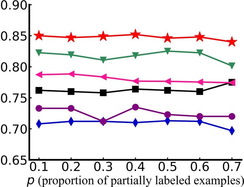
Under review as a conference paper at ICLR 2021

The generator Gn presented in the previous section provides a mechanism to generate noise labels
and denoise candidate label sets, but requires the true target label vector as its input. We propose
to use the outputs of the prediction network F to approximate the target true label vectors of the
training data for the purpose of denoising the candidate labels with Gn , while using the denoised
labels as the prediction target for F . Specifically, with the noise label generator Gn and the predictor
F , we perform partial label learning by minimizing the following classification loss on the training
data S:

                   min Lc (F, Gn ) = E ∼P            `c F (xi ), yi Gn (F (xi ), )                 (4)
                    F,Gn                   (xi ,yi )∼S

Although in the ideal case, the output vectors of Gn and F would be indicator label vectors, it
is error-prone and difficult for neural networks to output discrete values. To pursue more reliable
predictions and avoid overconfident outputs, we use Gn and F to predict the probability of each class
label being a noise label and the ground-truth label respectively. Hence the loss function `c (·, ·) in
Eq.(4) above denotes a mean square error loss between the predicted probability of each label being
the true label (through F ) and its denoised confidence of being a ground-truth label (through Gn ).

3.3   C ONDITIONAL F EATURE L EVEL DATA G ENERATION

With the noise label generation model and the prediction network above, the observed training data
in both the label and feature spaces are exploited to recognize the true labels and induce good
prediction models. Next, we incorporate a conditional data generator Gx (z, ) at the feature level to
map (denoised) label vectors in the label space into instances in the feature space, aiming to further
strengthen the mapping relations between data samples and the corresponding labels, enhance label
denoising and hence improve the partial label learning performance. Specifically, given a noise value
 sampled from a uniform distribution P and a one-hot label vector z sampled from a multinomial
distribution Pz , Gx (z, ) generates an instance in the feature space that is corresponding to label
z. Given the training label vectors in S denoised with Gn , the data generator Gx is also expected
to regenerate the corresponding training instances in the feature space. This assumption can be
captured using the following generation loss:

                            Lg (F, Gn , Gx ) = E (xi ,yi )∼S `g Gx (zi , 2 ), xi                  (5)
                                                  1 ,2 ∼P

                                      with zi = yi             Gn (F (xi ), 1 )
where zi denotes the denoised label vector for the i-th training instance, and `g (·, ·) is a mean square
error loss function.
Moreover, by introducing a discriminator Dx (x), which predicts how likely a given instance x is
real, we can deploy an adversarial learning scheme to learn the generator Gx through the following
minimax optimization problem with the WGAN loss:
               min max Lxadv (Gx , Dx ) = E(xi ,yi )∼S Dx (xi ) − E z∼Pz Dx (Gx (z, ))              (6)
               Gx    Dx                                                      ∼P

By playing a minimax game between Gx and Dx , this adversarial learning is expected to induce a
generator G∗x that can generate samples with the same distribution as the observed training instances.
Together with the generation loss in Eq.(5), we expect the mapping relation from label vectors to
samples induced by G∗x can be consistent with the observed data. Moreover, the consistency of the
mapping relation induced by Gx and the inverse mapping from samples to label vectors through the
prediction network F can be further strengthened by enforcing an auxiliary classification loss on the
generated data:

                             Lc0 (F, Gx ) = E z∼Pz `c0 F (Gx (z, )), z                            (7)
                                                ∼P

where `c0 (·, ·) can be a cross-entropy loss between the label prediction probability vector and the
sampled true label indicator vector.

3.4   L EARNING THE MGPLL M ODEL

By integrating the classification loss in Eq.(4), the adversarial losses in Eq.(2) and Eq.(6), the gener-
ation loss in Eq.(5) and the auxiliary classification loss in Eq.(7) together, MGPLL learning can be

                                                         5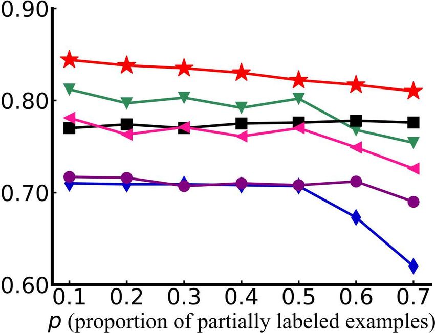
Under review as a conference paper at ICLR 2021

Table 1: Win/tie/loss counts of pairwise t-test (at 0.05 significance level) between MGPLL and each
comparison method.
                                                          MGPLL vs –
                                    SURE       PALOC        CLPL     PL-SVM          PL-KNN
            varying p [r = 1]      25/14/3     32/10/0      36/6/0    37/5/0          37/5/0
            varying p [r = 2]      27/13/2      33/9/0      33/9/0    38/4/0          35/7/0
            varying p [r = 3]      26/14/2     32/10/0     32/10/0    36/6/0          34/8/0
            varying  [p, r = 1]   25/17/0     30/12/0     32/10/0    35/7/0          33/9/0
            Total                  103/58/7    127/41/0    133/35/0 146/22/0         139/29/0

formulated as the following min-max optimization problem:
      min     max Lc (F, Gn )+Lnadv (Gn , Dn )+αLxadv (Gx , Dx )+βLg (F, Gn , Gx )+γLc0 (F, Gx )
    Gn ,Gx ,F Dn ,Dx
                                                                                                      (8)
where α, β and γ are trade-off hyperparameters. The learning of the overall model corresponds to a
minimax adversarial game. We develop a batch-based stochastic gradient descent algorithm to solve
it by conducting minimization over {Gn , Gx , F } and maximization over {Dn , Dx } alternatively.
The overall training algorithm is provided in the appendix.

4      E XPERIMENT
We conducted extensive experiments on both controlled synthetic PL datasets and real-world PL
datasets to investigate the empirical performance of the proposed model. In this section, we present
our experimental settings, comparison results and discussions.

4.1     E XPERIMENT S ETTING

Datasets The synthetic datasets are generated from six UCI datasets, ecoli, deter, vehicle, segment,
satimage and letter. From each UCI dataset, we generated synthetic PL datasets using three con-
trolling parameters p, r and , following the controlling protocol in previous studies (Wu & Zhang,
2018; Xu et al., 2019a; Lei & An, 2019). Among the three parameters, p controls the proportion
of instances that have noise candidate labels, r controls the number of false positive labels, and
controls the probability of a specific false positive label co-occurring with the true label. Under
different parameter configurations, multiple PL variants can be generated from each UCI dataset.
Given that both random noise labels and target label-dependent noise labels may exist in real-world
applications, we considered two types of settings. In the first type of setting, we consider random
noise labels with the following three groups of configurations: (I) r = 1, p ∈ {0.1, 0.2, · · ·, 0.7};
(II) r = 2, p ∈ {0.1, 0.2, · · ·, 0.7}; and (III) r = 3, p ∈ {0.1, 0.2, · · ·, 0.7}. In the second type of
setting, we consider the target label-dependent noise labels with the following configuration: (IV)
p = 1, r = 1,  ∈ {0.1, 0.2, · · ·, 0.7}. In total, the four groups of configurations provide us 168 (28
configurations × 6 UCI datasets) synthetic PL datasets.
We used five real-world PL datasets that are collected from several application domains, including
FG-NET (Panis & Lanitis, 2014) for facial age estimation, Lost (Cour et al., 2011), Yahoo! News
(Guillaumin et al., 2010) for automatic face naming in images or videos, MSRCv2 (Dietterich &
Bakiri, 1994) for object classification, and BirdSong (Briggs et al., 2012) for bird song classification.

Comparison Methods We compared the proposed MGPLL approach with the following PL meth-
ods, each configured with the suggested parameters according to the respective literature: PL-KNN
(Hüllermeier & Beringer, 2006), PL-SVM (Nguyen & Caruana, 2008), CLPL (Cour et al., 2011),
PALOC (Wu & Zhang, 2018), and SURE (Lei & An, 2019).

4.2     R ESULTS ON S YNTHETIC PL DATASETS

We conducted experiments on two types of synthetic PL datasets generated from the UCI datasets,
with random noise labels and target label-dependent noise labels, respectively. For each PL dataset,

                                                    6
Under review as a conference paper at ICLR 2021

       (a) vehicle                 (b) segment                 (c) satimage                  (d) letter

Figure 2: Test accuracy of each comparison method as  increases from 0.1 to 0.7 (with 100%
partially labeled examples [p = 1] and one false positive candidate label [r = 1]).

Table 2: Test accuracy (mean±std) of each comparison method on the real-world PL datasets. •/◦
indicates whether MGPLL is statistically superior/inferior to the comparison method on each dataset
(pairwise t-test at 0.05 significance level).
                     MGPLL         SURE            PALOC           CLPL            PL-SVM          PL-KNN
FG-NET               0.079±0.024   0.068±0.032     0.064±0.019     0.063±0.027     0.063±0.029     0.038±0.025 •
FG-NET(MAE3)         0.468±0.027   0.458±0.024     0.435±0.018 •   0.458±0.022     0.356±0.022 •   0.269±0.045 •
FG-NET(MAE5)         0.626±0.022   0.615±0.019     0.609±0.043 •   0.596±0.017 •   0.479±0.016 •   0.438±0.053 •
Lost                 0.798±0.033   0.780±0.036 •   0.629±0.056     0.742±0.038 •   0.729±0.042 •   0.424±0.036 •
MSRCv2               0.533±0.021   0.481±0.036 •   0.479±0.042 •   0.413±0.041 •   0.461±0.046 •   0.448±0.037 •
BirdSong             0.748±0.020   0.728±0.024 •   0.711±0.016 •   0.632±0.019 •   0.660±0.037 •   0.614±0.021 •
Yahoo! News          0.678±0.008   0.644±0.015 •   0.625±0.005 •   0.462±0.009 •   0.629±0.010 •   0.457±0.004 •

ten-fold cross-validation is performed and the average test accuracy results are recorded. Figure 2
presents the comparison results for the configuration setting (IV) on four datasets. We can see that
the proposed MGPLL consistently outperforms all the other methods.
To statistically study the significance of the performance gains achieved by MGPLL over the other
comparison methods, we conducted pairwise t-test at 0.05 significance level based on the compari-
son results of ten-fold cross-validation over all the 168 synthetic PL datasets obtained from all the
different configuration settings. The detailed win/tie/loss counts between MGPLL and each com-
parison method are reported in Table 1. From the results, we have the following observations: (1)
MGPLL achieves superior or at least comparable performance against PALOC, CLPL, PL-SVM and
PL-KNN in all cases, which is not easy given the comparison methods have different strengths across
different datasets. (2) MGPLL significantly outperforms PALOC, CLPL, PL-SVM and PL-KNN in
75.6%, 79.1%, 86.9% and 82.7% of the cases respectively, and produces ties in the remaining cases.
(3) MGPLL significantly outperforms SURE in 61.3% of the cases, achieves comparable perfor-
mance with SURE in 34.5% of the cases, while being outperformed by SURE in only 4.2% of the
cases. (4) On the PL datasets with target label-dependent noise labels, we can see that MGPLL
significantly outperforms SURE , PALOC, CLPL, PL-SVM, PL-KNN in 59.5%, 71.4%, 76.2%,
83.3%, 78.6% of the cases respectively. (5) It is worth noting that MGPLL is never significantly
outperformed by any comparison method on datasets with label-dependent noise labels. In sum-
mary, these results on the controlled PL datasets clearly demonstrate the effectiveness of MGPLL
for partial label learning under different settings.

4.3   R ESULTS ON R EAL -W ORLD PL DATASETS

We compared the proposed MGPLL method with the comparison methods on five real-world PL
datasets. For each dataset, ten-fold cross-validation is conducted. The mean test accuracy and
the standard deviation results are reported in Table 2. Moreover, statistical pairwise t-test at 0.05
significance level is conducted to compare MGPLL with each comparison method based on the
results of ten-fold cross-validation. The significance results are indicated in Table 2 as well. Note
that the average number of candidate labels (avg.#CLs) of FG-NET dataset is quite large, which
causes poor performance for all the comparison methods. For better evaluation of this facial age
estimation task, we employ the conventional mean absolute error (MAE) (Zhang et al., 2016) to
conduct two extra experiments. Two extra test accuracies are reported on the FG-NET dataset where

                                                       7
Under review as a conference paper at ICLR 2021

                Table 3: Comparison results of MGPLL and its five ablation variants.
                   MGPLL         CLS-w/o-advn    CLS-w/o-advx    CLS-w/o-g     CLS-w/o-aux   CLS
FG-NET             0.079±0.024   0.061±0.024     0.072±0.020     0.068±0.029   0.076±0.022   0.057±0.016
FG-NET(MAE3)       0.468±0.027   0.430±0.029     0.451±0.032     0.436±0.038   0.456±0.033   0.420±0.420
FG-NET(MAE5)       0.626±0.022   0.583±0.055     0.605±0.031     0.590±0.045   0.612±0.044   0.570±0.034
Lost               0.798±0.033   0.623±0.037     0.754±0.032     0.687±0.026   0.782±0.043   0.609±0.040
MSRCv2             0.533±0.021   0.472±0.030     0.480±0.038     0.497±0.031   0.526±0.036   0.450±0.037
BirdSong           0.748±0.020   0.728±0.010     0.732±0.011     0.716±0.011   0.742±0.024   0.674±0.016
Yahoo! News        0.678±0.008   0.645±0.008     0.675±0.009     0.648±0.014   0.671±0.012   0.610±0.015

a test sample is considered to be correctly predicted if the difference between the predicted age and
the ground-truth age is less than 3 years (MAE3) or 5 years (MAE5). From Table 2 we have the
following observations: (1) Comparing with all the other five PL methods, MGPLL consistently
produces the best results on all the datasets, with remarkable performance gains in many cases. For
example, MGPLL outperforms the best alternative comparison methods by 5.2%, 3.4% and 2.0%
on MSRCv2, Yahoo! News and Birdsong respectively. (2) Out of the total 35 comparison cases (5
comparison methods × 7 datasets), MGPLL significantly outperforms all the comparison methods
across 77.1% of the cases, and achieves competitive performance in the remaining 22.9% of cases.
(3) It is worth noting that the performance of MGPLL is never significantly inferior to any other
comparison method. These results again validate the efficacy of the proposed method.

4.4   A BLATION S TUDY

The objective function of MGPLL contains five loss terms: classification loss, adversarial loss at
the label level, adversarial loss at the feature level, generation loss and auxiliary classification loss.
To assess the contribution of each part, we conducted an ablation study by comparing MGPLL
with the following ablation variants: (1) CLS-w/o-advn, which drops the adversarial loss at the
label level. (2) CLS-w/o-advx, which drops the adversarial loss at the feature level. (3) CLS-
w/o-g, which drops the generation loss. (4) CLS-w/o-aux, which drops the auxiliary classification
loss. (5) CLS, which only uses the classification loss by dropping all the other loss terms. The
comparison results are reported in Table 3. We can see that comparing to the full model, all five
variants produce inferior results in general and have performance degradations to different degrees.
This demonstrates that the different components in MGPLL all contribute to the proposed model to
some extend. From Table 3, we can also see that the variant CLS-w/o-advn has a relatively larger
performance degradation by dropping the adversarial loss at the label level, while the variant CLS-
w/o-aux has a small performance degradation by dropping the auxiliary classification loss. This
makes sense as by dropping the adversarial loss for learning noise label generator, the generator
can produce poor predictions and seriously impact the label denoising of the MGPLL model. This
suggests that our non-random noise label generation through adversarial learning is a very effective
and important component for MGPLL. For CLS-w/o-aux, as we have already got the classification
loss on real data, it is reasonable to see that the auxiliary classification loss on generated data can
help but is not critical. Overall, the ablation results suggest that the proposed MGPLL is effective.

5     C ONCLUSION

In this paper, we proposed a novel multi-level generative model, MGPLL, for partial label learning.
MGPLL uses a conditional label level generator to model the target label dependent non-random
noise label appearances, which directly performs candidate label denoising, while using a condi-
tional feature level generator to generate data samples from denoised label vectors. Moreover, a
prediction network is incorporated to predict the denoised true label of each instance from its input
features, which forms bi-directional inverse mappings between labels and features, together with
the data feature generator. The adversarial learning of the overall model simultaneously identifies
true labels of the training instances from both the observed data features and the observed candidate
labels, while inducing accurate prediction networks that map input feature vectors to (denoised) true
label vectors. We conducted extensive experiments on real-world and synthesized PL datasets. The
proposed MGPLL model demonstrates the state-of-the-art PL performance.

                                                    8
Under review as a conference paper at ICLR 2021

R EFERENCES
Eric Arazo, Diego Ortego, Paul Albert, Noel E O’Connor, and Kevin McGuinness. Unsupervised
  label noise modeling and loss correction. arXiv preprint arXiv:1904.11238, 2019.
Martin Arjovsky, Soumith Chintala, and Léon Bottou. Wasserstein generative adversarial networks.
 In Proceedings of the International Conference on Machine Learning (ICML), 2017.
Forrest Briggs, Xiaoli Z Fern, and Raviv Raich. Rank-loss support instance machines for miml
  instance annotation. In Proceedings of the ACM SIGKDD international conference on Knowledge
  discovery and data mining (KDD), 2012.
Jingwen Chen, Jiawei Chen, Hongyang Chao, and Ming Yang. Image blind denoising with gen-
   erative adversarial network based noise modeling. In Proceedings of the IEEE Conference on
   Computer Vision and Pattern Recognition, pp. 3155–3164, 2018.
Timothee Cour, Ben Sapp, and Ben Taskar. Learning from partial labels. Journal of Machine
  Learning Research, 12(May):1501–1536, 2011.
Thomas G Dietterich and Ghulum Bakiri. Solving multiclass learning problems via error-correcting
  output codes. Journal of artificial intelligence research, 2:263–286, 1994.
Qi Dou, Cheng Ouyang, Cheng Chen, Hao Chen, and Pheng-Ann Heng. Unsupervised cross-
  modality domain adaptation of convnets for biomedical image segmentations with adversarial
  loss. arXiv preprint arXiv:1804.10916, 2018.
Jun-Peng Fang and Min-Ling Zhang. Partial multi-label learning via credible label elicitation. In
  Proceedings of the AAAI Conference on Artificial Intelligence, volume 33, pp. 3518–3525, 2019.
Lei Feng and Bo An. Leveraging latent label distributions for partial label learning. In International
  Joint Conference on Artificial Intelligence (IJCAI), 2018.
Lei Feng and Bo An. Partial label learning by semantic difference maximization. In International
  Joint Conference on Artificial Intelligence (IJCAI), 2019.
Chen Gong, Tongliang Liu, Yuanyan Tang, Jian Yang, Jie Yang, and Dacheng Tao. A regularization
  approach for instance-based superset label learning. IEEE transactions on cybernetics, 48(3):
  967–978, 2018.
Ian Goodfellow, Jean Pouget-Abadie, Mehdi Mirza, Bing Xu, David Warde-Farley, Sherjil Ozair,
  Aaron Courville, and Yoshua Bengio. Generative adversarial nets. In Advances in Neural Infor-
  mation Processing Systems (NeurIPS), 2014a.
Ian Goodfellow, Jean Pouget-Abadie, Mehdi Mirza, Bing Xu, David Warde-Farley, Sherjil Ozair,
  Aaron Courville, and Yoshua Bengio. Generative adversarial nets. In Advances in neural infor-
  mation processing systems, 2014b.
Matthieu Guillaumin, Jakob Verbeek, and Cordelia Schmid. Multiple instance metric learning from
 automatically labeled bags of faces. In European Conference on Computer Vision (ECCV), 2010.
Eyke Hüllermeier and Jürgen Beringer. Learning from ambiguously labeled examples. Intelligent
  Data Analysis, 10(5):419–439, 2006.
Rong Jin and Zoubin Ghahramani. Learning with multiple labels. In Advances in neural information
  processing systems (NeurIPS), 2003.
Feng Lei and Bo An. Partial label learning with self-guided retraining. In AAAI Conference on
  Artificial Intelligence (AAAI), 2019.
Liping Liu and Thomas G Dietterich. A conditional multinomial mixture model for superset label
  learning. In Advances in neural information processing systems, pp. 548–556, 2012.
Jie Luo and Francesco Orabona. Learning from candidate labeling sets. In Advances in Neural
   Information Processing Systems (NeurIPS), 2010.

                                                  9
Under review as a conference paper at ICLR 2021

Nam Nguyen and Rich Caruana. Classification with partial labels. In Proceedings of the ACM
  SIGKDD international conference on Knowledge discovery and data mining (KDD), 2008.
Gabriel Panis and Andreas Lanitis. An overview of research activities in facial age estimation using
  the fg-net aging database. In European Conference on Computer Vision (ECCV), 2014.
Cai-Zhi Tang and Min-Ling Zhang. Confidence-rated discriminative partial label learning. In AAAI
  Conference on Artificial Intelligence (AAAI), 2017.
Kiran K Thekumparampil, Ashish Khetan, Zinan Lin, and Sewoong Oh. Robustness of conditional
  gans to noisy labels. In Advances in neural information processing systems, pp. 10271–10282,
  2018.
Tijmen Tieleman and Geoffrey Hinton. Lecture 6.5-rmsprop: Divide the gradient by a running
   average of its recent magnitude. COURSERA: Neural networks for machine learning, 4(2):26–
   31, 2012.
Deng-Bao Wang, Li Li, and Min-Ling Zhang. Adaptive graph guided disambiguation for partial
  label learning. In Proceedings of the 25th ACM SIGKDD International Conference on Knowledge
  Discovery & Data Mining, pp. 83–91, 2019a.
Haobo Wang, Weiwei Liu, Yang Zhao, Chen Zhang, Tianlei Hu, and Gang Chen. Discriminative
  and correlative partial multi-label learning. In Proceedings of the Twenty-Eighth International
  Joint Conference on Artificial Intelligence, IJCAI, pp. 10–16, 2019b.
Xuan Wu and Min-Ling Zhang. Towards enabling binary decomposition for partial label learning.
  In International Joint Conference on Artificial Intelligence (IJCAI), 2018.
Ming-Kun Xie and Sheng-Jun Huang. Partial multi-label learning. In Thirty-Second AAAI Confer-
 ence on Artificial Intelligence, 2018.
Ning Xu, Jiaqi Lv, and Xin Geng. Partial label learning via label enhancement. In AAAI Conference
  on Artificial Intelligence (AAAI), 2019a.
Yilun Xu, Peng Cao, Yuqing Kong, and Yizhou Wang. L dmi: A novel information-theoretic loss
  function for training deep nets robust to label noise. In Advances in Neural Information Process-
  ing Systems, pp. 6222–6233, 2019b.
Yan Yan and Yuhong Guo. Partial label learning with batch label correction. In AAAI Conference
  on Artificial Intelligence (AAAI), 2020.
Yao Yao, Chen Gong, Jiehui Deng, Xiuhua Chen, Jianxin Wu, and Jian Yang. Deep discriminative
  cnn with temporal ensembling for ambiguously-labeled image classification. In AAAI Conference
  on Artificial Intelligence (AAAI), 2020.
Fei Yu and Min-Ling Zhang. Maximum margin partial label learning. In Asian Conference on
  Machine Learning, pp. 96–111, 2016.
Zinan Zeng, Shijie Xiao, Kui Jia, Tsung-Han Chan, Shenghua Gao, Dong Xu, and Yi Ma. Learning
  by associating ambiguously labeled images. In Proceedings of the IEEE Conference on Computer
  Vision and Pattern Recognition (CVPR), 2013.
Min-Ling Zhang and Fei Yu. Solving the partial label learning problem: An instance-based ap-
 proach. In International Joint Conference on Artificial Intelligence (IJCAI), 2015.
Min-Ling Zhang, Bin-Bin Zhou, and Xu-Ying Liu. Partial label learning via feature-aware disam-
 biguation. In Proceedings of the ACM SIGKDD International Conference on Knowledge Discov-
 ery and Data Mining (KDD), 2016.
Min-Ling Zhang, Fei Yu, and Cai-Zhi Tang. Disambiguation-free partial label learning. IEEE
 Transactions on Knowledge and Data Engineering, 29(10):2155–2167, 2017.
Zhengli Zhao, Dheeru Dua, and Sameer Singh. Generating natural adversarial examples. arXiv
  preprint arXiv:1710.11342, 2017.
Zhi-Hua Zhou. A brief introduction to weakly supervised learning. National Science Review, 5(1):
  44–53, 2018.

                                                10
Under review as a conference paper at ICLR 2021
Algorithm 1 Minibatch stochastic gradient descent.
Input: S : the PL training set; α, β, γ: the trade-off hyperparameters;
. c: the clipping parameter; m: minibatch size.
for number of training iterations do
Sample a minibatch B = {(xi , yi )}m i=1 of m samples from S.
Sample m noise values {1 , · · · , i , · · · , m } from a prior P ().
Sample m label vectors {z1 , · · · , zi , · · · , zm } from a prior Pz .
Update Dn , Dx by ascending their stochastic gradients:
m
1 X n o
∇ΘDn ,Dx Dn (yi ) − Dn (Gn (zi , i ) ⊕ zi ) + α Dx (xi ) − Dx (Gx (zi , i ))
m i=1
Perform WGAN adjustment: ΘDn ,Dx ← clip(ΘDn ,Dx , −c, c)
Sample m noise values {1 , · · · , i , · · · , m } from a prior P ().
Update Gn , Gx , F by stochastic gradient descent:
m
1 X `c (F (xi ), yi Gn (F (xi ), i )) − Dn(Gn (zi , i ) ⊕ zi ) − αDx (Gx (zi , i ))+
∇ΘGn ,Gx ,F
m β`g Gx yi Gn (F (xi ), i ), i , xi + γ`c0 F (Gx (zi , i ), zi )
i=1
end for
Table 4: Characteristics of the UCI datasets (left side) and the real-world PL datasets (right side).
Dataset #Example #Feature #Class Dataset #Example #Feature #Class avg.#CLs
ecoli 336 7 8 FG-NET 1,002 262 78 7.48
deter 358 23 6 Lost 1,122 108 16 2.23
vehicle 846 18 4 MSRCv2 1,758 48 23 3.16
segment 2310 18 7 BirdSong 4,998 38 13 2.18
satimage 6,345 36 7 Yahoo! News 22,991 163 219 1.91
letter 20,000 16 26
A A PPENDIX
A.1 T HE OVERALL T RAINING A LGORITHM
The overall training algorithm for solving the formulated min-max optimization problem in Eq.(8)
is outlined in Algorithm 1.
A.2 T HE C HARACTERISTICS OF THE DATASETS
The characteristics of the UCI datasets and the real-world PL datasets are summaized in Table 4.
A.3 I MPLEMENTATION D ETAILS
The proposed MGPLL model has five component networks, all of which are designed as multilayer
perceptrons with Leaky ReLu activation for the middle layers. The noise label generator is a four-
layer network with sigmoid activation in the output layer. The conditional data generator is a five-
layer network with tanh activation in the output layer, while batch normalization is deployed in its
three middle layers. The predictor is a three-layer network with softmax activation in the output
layer. Both the noise label discriminator and the data discriminator are three-layer networks without
activation in the output layer. We used the RMSProp (Tieleman & Hinton, 2012) optimizer in our
implementation and the mini-batch size m is set to 32. We selected the hyperparameters α, β and
γ from {0.001, 0.01, 0.1, 1, 10} in a heuristic way based on the classification loss value Lc in the
training objective function; that is, we chose their values that lead to the smallest training Lc loss.
11Under review as a conference paper at ICLR 2021
(a) ecoli (b) deter (c) vehicle
(d) segment (e) satimage (f) letter
Figure 3: Test accuracy of each comparison method changes as (co-occurring probability of the
coupling label) increases from 0.1 to 0.7 (with 100% partially labeled examples [p = 1] and one
false positive candidate label [r = 1]).
(a) ecoli (b) deter (c) vehicle
(d) segment (e) satimage (f) letter
Figure 4: Test accuracy of each comparison method changes as p (proportion of partially labeled
examples) increases from 0.1 to 0.7 (with one false positive candidate label [r = 1]).
A.4 M ORE R ESULTS ON S YNTHETIC PL DATASETS
We conducted experiments on two types of synthetic PL datasets generated from the UCI datasets,
with random noise labels and target label-dependent noise labels, respectively. For each PL dataset,
ten-fold cross-validation is performed and the average test accuracy results are recorded. First we
study the comparison results over the synthetic PL datasets with target label-dependent noise labels
under the PL configuration setting (IV). In this setting, a specific label is selected as the coupled label
that co-occurs with the ground-truth label with probability , and any other label can be randomly
chosen as a noisy label with probability 1 − . Figure 3 presents the comparison results for the
configuration setting (IV), where increases from 0.1 to 0.7 with p = 1 and r = 1. From Figure
3 we can see that the proposed MGPLL produces impressive results. It consistently outperforms
12Under review as a conference paper at ICLR 2021
(a) ecoli (b) deter (c) vehicle
(d) segment (e) satimage (f) letter
Figure 5: Test accuracy of each comparison method changes as p (proportion of partially labeled
examples) increases from 0.1 to 0.7 (with two false positive candidate label [r = 2]).
(a) ecoli (b) deter (c) vehicle
(d) segment (e) satimage (f) letter
Figure 6: Test accuracy of each comparison method changes as p (proportion of partially labeled
examples) increases from 0.1 to 0.7 (with three false positive candidate label [r = 3]).
all the other methods across different values on four datasets, vehicle, segment, satimage and
letter, while achieving remarkable performance gains on segment and satimage. On the other two
datasets, ecoli and deter, MGPLL also produces the best results in most cases and remains to be
the most effective method. By contrast, the performance of the other comparison methods varies
largely across different datasets. For example, CLPL and SURE demonstrate good performance on
ecoli, deter and vehicle, but presents inferior results than PL-KNN in many cases of the other three
datasets. PALOC and PL-SVM have the same drawback of producing poor results on some datasets.
Our proposed MGPLL demonstrates good overall performance across these varying cases.
We also conducted experiments on the PL datasets with random noise labels produced under the
PL configuration settings (I), (II) and (III). The comparison results in these three sets of configura-
tions are reported in Figure 4, Figure 5 and Figure 6 respectively. From these figures we can see
13Under review as a conference paper at ICLR 2021
Figure 7: Parameter sensitivity analysis for MGPLL on the Lost and MSRCv2 datasets.
that the proposed MGPLL (with noise label generator Gn ()) achieves similar positive comparison
results as in the configuration setting (IV). In particular, the proposed method achieves remarkable
performance gains on four of the overall six datasets, segment, satimage, vehicle and letter.
A.5 PARAMETER S ENSITIVITY A NALYSIS
We also conducted parameter sensitivity analysis on two real-world PL datasets BirdSong and Ya-
hoo! News datasets to study how the trade-off hyperparameters α, β and γ influence the performance
of MGPLL. We conducted the experiments by using different combination settings of the α, η and
γ values from {0.001, 0.01, 0.1, 1, 10}. We vary each parameter’s value by keeping the other two
fixed at their best setting. Note that a larger value for α, β and γ will provide larger weight to the
feature level WGAN loss, generation loss and auxiliary classification loss respectively.
The three figures in Figure 7 report the average test results as well as standard deviations for different
α, β and γ values respectively. We can see that when α is very small, the performance of MGPLL is
not very good since the feature level WGAN loss is not allowed to contribute much to the learning.
With the increase of α, the performance improves, which suggests that the WGAN loss is important.
When α is too large, the performance degrades as the WGAN loss dominates. This is reasonable
since the WGAN loss is expected to help the predictive model, rather than dominate the learning
process. A similar phenomenon can be observed for γ. For the parameter β, the proposed method
performs bad when β is very small. With the increase of β, the performance of MGPLL improves
and remains relatively stable in a broader range, i.e., β ∈ [0.01, 1]. It shows that the proposed model
is not very sensitivity to the β parameter within the considered range of values.
14You can also read