Manual for installation and usage of R-php - Angelo M. Mineo & Alfredo Pontillo Versione n. 0.99a
←
→
Page content transcription
If your browser does not render page correctly, please read the page content below
Manual for installation and usage of R-php
                 Versione n. 0.99a

       Angelo M. Mineo & Alfredo Pontillo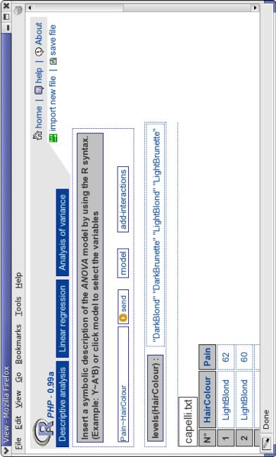
1

Presentation
R-php is a project developed inside the Department of Statistical and Mathemat-
ical Sciences “Silvio Vianelli” of the University of Palermo (Italy) and has as goal
the realization of a web-oriented statistical software, i.e. a software which the final
user reaches through Internet and requires for the running only the installation of a
browser, that is a program for the hypertext visualization (examples of browser are:
Explorer, Mozilla, Firefox, Opera, and so on).
   R-php is an open-source project with the code released by the authors and can
be freely installed (see paragraph 1.1)
   The idea to project a statistical software that can be used through Internet comes
out from the following considerations: it is an ascertained fact that the growing
spread of Internet and the request of new services from its users has changed and
still is radically changing the way to access the daily use structures (work, study, and
so on); by now the most of information and services goes through the Web and the
software philosophy goes to the same direction; on the database management software
an example is the package PhpMyAdmin that is a via web graphical interface of
MySQL, the database management system more used for web-oriented applications;
on the business field another example of use of the Web is the develop of home-banking
services.
   In general, the trend on producing software that are installed on a single computer
is going down in favour of software that can be used through a connession to Internet
and a browser.
   A main feature of R-php is that all the statistical analyses exploit as “engine” the
open-source statistical programming environment R, that is more and more used not
only from the academic world, but also from consulting firms (Marc Scwatz, 2004,
The Decision to Use R: a cosulting business perspective, R News, Vol. 4(1), pp.
2-5). Then R-php is classifiable among the web projects dedicated to R. Beyond
this project, there are others such as: R-web, R-PHP, and so on (see the web page
http://http://franklin.imgen.bcm.tmc.edu/R.web.servers). Shortly, the main
difference between R-php and the previously cited projects consists in the presence

2

of an interactive module (R-php point-and-click ) inside R-php, that allows to make
some of the main statistical analyses without the user has to know the statistical
environment R.
   The potential users of R-php are several: let’s think about, for example, students
either inside didactic facilities, such as informatic laboratories, or at home through a
simple Internet connection, or a possible user that does not know and wants not to
know a programming environment as R, but wants to make some simple statistical
analyses without buying the license of a commercial statistical software.
Chapter 1

Main features of R-php

1.1      Guide to the installation of a R-php server
In this section we shall see how to install R-php on an Apache server, refering
to the next paragraphs for a more detailed description of the needed software for
a correct running of R-php. In a simple manner, with no loss of generality, to
point out the necessary steps for the installation, we shall refer to a LAMP system
(Linux, Apache, MySQL, PHP), i.e. a computer with a Linux operating system,
with Apache web server, with MySQL and PHP. Downloaded the R-php-xxx.tar.gz
source from the web site http://dssm.unipa.it/R-php, or from http://r-php.
homelinux.net, we have to follow these steps:

  1. Obtaining the super user (root) privilege with the command su.

  2. Copying the source on the Apache root: for example, by opening a console
      and by going to the directory where the file R-php-xxx.tar.gz is, it is sufficient
      to execute the following command:

        • for a Redhat based distribution

           ]\# cp R-php-xxx.tar.tgz /var/www/html/

        • for a Debian distribution

                                           3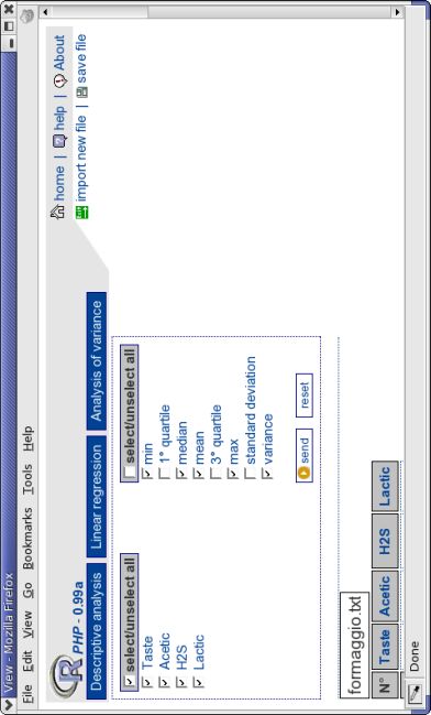
CHAPTER 1. MAIN FEATURES OF R-PHP                                                4

          ]\# cp R-php-xxx.tar.tgz /var/www/

  3. Extracting the R-php-xxx.tar.gz file, for example with the following command:

     ]\# tar xvzf R-php-xxx.tar.gz

     Now, the user can find the R-php-xxx directory starting from the root of the
     Apache server: this directory includes all the software.

  4. Entering the R-php-xxx directory with the following command:

     ]\# cd R-php-xxx

     This directory has the following components:

       • COPYNG (file containing the user license);
       • Doc (directory containing the documentation);
       • include (directory containing the configuration files);
       • index.html (main page);
       • R (directory containing R-php base);
       • README (file containing some beginning information about the soft-
          ware);
       • R-gui (directory containing R-php Point and Click );

  5. Entering the include directory with the following command:

     ]\# cd include

  6. Editing (by using, for example, vi) the conn.php file, by modifying the fields
     with the necessary data for the access to MySQL (user id and password).

     ]\# vi conn.php

   Now, it is sufficient loading with a browser the site http://localhost/R-php-xxx/
or the site http://your-domain/R-php-xxx, to run R-php.
CHAPTER 1. MAIN FEATURES OF R-PHP                                                       5

1.2      Description of R-php
In this paragraph we shall illustrate the needed software for the implementation of a
R-php server and the used code for the running of the two considered modules. We
want to point out that all the used software is open-source.

1.2.1     Needed software
For a correct running of R-php it is necessary installing the following software on
the server:

   • Apache:
      The Apache Httpd server:

        – is a powerful, flexible, HTTP/1.1 compliant web server;
        – implements the latest protocols;
        – is highly configurable and extensible with third-party modules;
        – can be customized by writing “modules” using the Apache module API;
        – provides full source code and comes with an unristrictive license;
        – runs on Windows NT/9X, Netware 5.X and above, OS/2 and most
              versions of UNIX, as well as several other operating systems;
        – is actively being developed;
        – implements many frequently requested features, including:
               ∗ DBM databases for authentication, that allows to set up easily password-
                  protected pages with enormous numbers of authorized users, without
                  bogging down the server;
               ∗ customized responses to errors; indeed, it allows to set up files or even
                  CGI scripts, which are returned by the server in response to errors and
                  problems;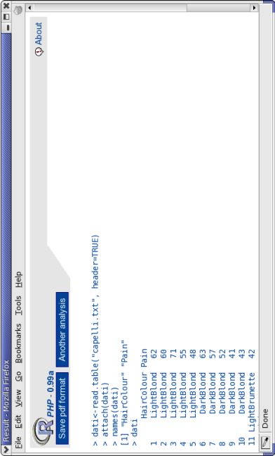
CHAPTER 1. MAIN FEATURES OF R-PHP                                                 6

         ∗ Multiple DirectoryIndex directives, that instructs the server which files
            have to consider when a directory URL is requested, whichever it finds
            in the directory;
         ∗ virtual hosts, that is a much requested feature, sometimes known as
            “multi-homed-servers”; this feature allows the server to distinguish
            between requests made to different IP addresses or names “mapped”
            to the same machine;
         ∗ Configurable reliable piped logs.

   Nowadays, Apache is considered the most efficient, fast and functional Web
   server; according to the data given by the Netcraft Web Server Survay (http:
   //news.netcraft.com/archives/web_server_survey.html) Apache is the
   more used Web server all around the World, with a pecentage of use equal to
   68.43 % (this result is referred to Jenuary 2005). For a comparison among the
   more common used Web server see figure 1.1.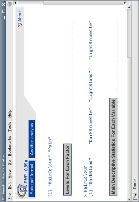
CHAPTER 1. MAIN FEATURES OF R-PHP                                         7

       Figure 1.1: Statistics on the diffusion of the main Web servers.
CHAPTER 1. MAIN FEATURES OF R-PHP                                                     8

  • R
   R is a language and environment for statistical computing and graphics; it is
   a GNU project which is similar to the S language and environment which was
   developed at BELL Laboratories, formerly AT&T and now Lucent Technologies
   by John Chambers and colleagues. R can be considered as a different imple-
   mentation of S. There are some important differences, but much code written
   for S runs unaltered under R. R provides a wide variety of statistical (linear
   and nonlinear modelling, classical statistical tests, time-series analysis, classifi-
   cation, clustering, ...) and graphical techniques, and is highly extensible. The
   S language is often the vehicle of choice for research in statistical methodology
   and R provides an Open Source route to participation in that activity. One of
   R’s strengths is the ease with which well-designed publication-quality plots can
   be produced, including mathematical symbols and formulae where needed. R
   compiles and runs on a wide variety of UNIX platforms and similar systems
   (including FreeBSD and Linux), Windows and MacOS. R is an integrated
   suite of software facilities for data manipulation, calculation and graphical dis-
   play and includes:

        – an effective data handling and storage facility;
        – a suite of operators for calculations on arrays, in particular matrices;
        – a large, coherent, integrated collection of intermediate tools for data anal-
          ysis;
        – graphical facilities for data analysis and display either on-screen or on
          hardcopy;
        – a well-developed, simple and effective programming language which in-
          cludes conditionals, loops, user-defined recursive functions and input/output
          facilities.

   The term “environment” is intended to characterize it as a fully planned and
   coherent system, rather than an incremental accretion of very specific and in-
   flexible tools, as is frequently the case with other data analysis software.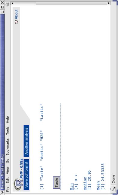
CHAPTER 1. MAIN FEATURES OF R-PHP                                                   9

  • PHP
   PHP is an HTML-embedded scripting language, i.e. a language that allows to
   insert code executable inside HTML pages. Much of its syntax is borrowed
   from C, Java and Perl with a couple of unique PHP-specific features thrown
   in. The goal of PHP is to allow web developers to write dynamically generated
   pages quickly. PHP stands for PHP Hypertext Preprocessor and then its name
   is a so called recursive acronym.

  • MySQL
   MySQL is a relational database management system. The main feature of a
   relational database is the capacity to store data in separate structures, called
   tables, rather than putting all the data in one big area. The SQL part of
   MySQL is acronym of Structure Query Language, which is the most common
   language used to access database. The MySQL database server is the most
   popular open-source database in the World; its diffusion is due to the great
   speed and flexibility; it is exactly the speed to access data that makes MySQL
   suitable for the implementation of Web applications.

  • ImageMagick
   ImageMagick is a collection of tools and libraries to manipulate an image.
   ImageMagick can read, write, and manipulate image in any of the more pop-
   ular image formats, including .gif, .jpeg, .png e .pdf; moreover, you can create
   .gif’s dynamically making it suitable for Web applications. Here are just a few
   examples of what ImageMagick can do:

     – Convert an image from one format to another;
     – Resize, rotate, sharpen, color reduce, or add special effects to an image;
     – Create thumbnails;
     – Turn a group of images into a .gif animation sequence;
     – Draw shapes or text on an image;
     – Decorate an image with a border or frame;
CHAPTER 1. MAIN FEATURES OF R-PHP 10
– Describe the format and characteristics of an image.
The main feature of ImageMagick, that makes it a necessary tool to manip-
ulate images also for Web applications, it is the possibility to make the above
mentioned (and not only) operations by shell, for example BASH 1 ).
As it is known, R has several commands to create images of different formats
(.png, .jpeg, .ps, and so on), but in the base module of R-php the use of
ImageMagick has been more easily manageable. Moreover, under UNIX the
R’s png device uses the X11 driver, which is a problem in “batch mode” or
for remote operation. The use of ImageMagick in the base module has been
extended also to the point-and-click module of R-php. Then, R, invocated in
“batch mode”, gives graphs in .ps format; following, it is reported the PHP
code to manipulate and convert the .ps file in a “web-compatible” format by
using ImageMagick:
exec("convert ./pages/tmp/$temp/Rplots.ps ./pages/tmp/$temp/R.png");
exec("convert -antialias -rotate 90 $fn ./pages/tmp/$temp/$nn.png");
• htmldoc
htmldoc is a program that generates indexed .html, Adobe PostScript, and
.pdf files from .html ”source” files. htmldoc includes a simple GUI (Grafical
User Interface) to manage your .html files and automatically (re)generate files
for viewing and printing. htmldoc can also be used on your web server to
generate files “on-the-fly”.
For the above described software it is advisable to have the last versions and anyway
it is necessary having installed: for PHP a version from the 4.3.0., for R a version
from 2.0.0.
1
Bourn Again SHellCHAPTER 1. MAIN FEATURES OF R-PHP 11
1.2.2 Description of the first module (R-php base)
When the user enters the home page of this module, a temporary directory is created;
the name of this directory is generated by this portion of code:
$unico = substr(uniqid("5555"),-5);
$time = time();
$max = mktime(6, 0, 0, 1, 1, 1970);
$temp = $unico."_".$time;
According to the implemented code, first it is generated a pseudo-random string of
alpha-numeric characters, to which is associated the UNIX timestamp. Into this
temporary directory we have all the user generated files that are created during the
current work session; this guarantees the multiuse, i.e. the concurrent use of more
users, without creating confusion between the files created in different concurrent
sessions. This feature of R-php does not seem it is implemented in other similar
systems. The maximum number of concurrent users does not depend on R-php, but
on the set up of the hosting Apache server. Following, there is the PHP code that
compares the current UNIX timestamp with that present in the temporary directory
name and deletes those directories present in the server for more than six hours: this
allows to avoid a great number of temporary directories into the server:
foreach(glob("./pages/tmp/*") as $dir){
$time_scad_temp = explode("_", $dir);
$control = $time - $time_scad_temp[1];
if($control>=$max){
delfile("$dir/*");
rmdir("$dir");
}
}
mkdir("pages/tmp/$temp", 777);
chmod("pages/tmp/$temp", 0777);CHAPTER 1. MAIN FEATURES OF R-PHP 12
The first module of R-php allows in a textarea the immission of portions of R
code that is transcripted in a text file. Following, there is the sequence of PHP
instructions that allow this operation:
$nomefile = "codice.txt";
$fp = fopen("./pages/tmp/$temp/$nomefile", "w")
or die("impossibile aprire file");
fputs ( $fp, "$codice") or die("impossibile scrivere");
fclose($fp);
As it is known, R has commands that permit the interactions with the operatimg
system of the used computer; this could be dangerous in an environment like this one,
because an outer user could input (voluntarily or not) harmful commands. To avoid
this drawback, we have decided to implement a control structure that does not allow
the use of a set of commands that we think are dangerous for the server safety. These
commands are reported in a MySQL database, containing also a short description
of what the banned command would do. It is clear that the user, interested to install
R-php on an own server, can modify this list of commands in any time. For more
safety, this control structure works first “client-side” in javascript and next (only if
the first control is evaded) also “server-side” in PHP.
For the data input, besides the possibility to insert the data at hand through
the R commands, there is the chance to import the data from a text file. From a
technical point of view, this operation is an “upload” on the server, by using the
following sequence of PHP commands:
if(isset($HTTP_POST_VARS[upFile]) and $HTTP_POST_VARS[upFile] = "yes"){
include("./include/temp.php");
$nomeFile = pulisci($HTTP_POST_FILES[’file’][’name’]);
move_uploaded_file($HTTP_POST_FILES[’file’][’tmp_name’],
"./pages/tmp/$_SESSION[temp]/$nomeFile");
}CHAPTER 1. MAIN FEATURES OF R-PHP 13
The R commands, that are in the previously created file, are processed from R
that is invocated by PHP in “batch mode”. The command that makes this operation
is the following:
exec(R --no-save -q < codice.txt > output 2>&1);
R, invocated in “batch mode”, gives the output in two formats: the former is
textual with the requested analysis, the latter in .ps format containing the possible
graphs. At this point, the two files are treated in two different ways:
• the text file is simply formatted (by using the style-sheet) to make it more
readable;
• the .ps format file is split to obtain a file for each image; then each image is
converted in a more suitable format for the Web visualization (.png format);
these operations are done with ImageMagick.
In the final phase the output, with all the graphs, is visualized in a new window.
In this window there is the possibility for the user to save the output in .pdf format
by means of the software htmldoc, or the user can decide to save only the desidered
graphs produced in the work session.
1.2.3 Description of the second module (R-php point-and-
click)
The R-php module, that we describe in this paragraph, is not a simple R web
interface, but it has all the characteristics of a GUI; this part makes R-php a new
project on respect to the other similar project.
The organization of the concurrent sessions of this module is the same of the
organization of the R-php base module, described in the previous paragraph.
About the data input, that is the first step on the use of R-php point-and-click,
it is done by loading an ASCII file from the user computer. Then, the file content is
visualized in a new page as a “spreadsheet”; this data set is managed by MySQL:CHAPTER 1. MAIN FEATURES OF R-PHP 14
this allows to make some interactive operations on the data: for example, it is possible
to modify the variable names or a value in each cell of the “spreadsheet”; following,
there is the PHP and MySQL code to modify a cell value:
$sql = "UPDATE $temp SET var$v = ’$val’ where id=’$r’";
mysql_query ($sql, $conn);
Loaded the data set, it is possible to choose what kind of analysis we have to
perform among those proposed. Each analysis can be performed by means of a GUI;
in this GUI they are chosen the analysis options that the user want to set up; these
options are coded in R and this code is processed by the R environment. With a
greater detail, this phase follows this steps:
1. the code is put in an ASCII file that is the R input; this operation is the same
of that one described for the base module;
2. the database containing the data is exported in an ASCII file; following, there
is the used code:
exec("mysqldump -T ./pages/tmp/$temp --fields-terminated-by=’ ’
R $temp -u’$user’ -p’$pass’");
3. R, invocated in “batch mode”, processes the code that is in the previously
created file;
4. R gives the output in two files: the first one (in text format) containg the textual
part of the analysis, the secon one (in .ps format) containing the graphs;
5. the ASCII file is formatted according to the Web standards;
6. the .ps file is first split in more files and then handled and converted by Im-
ageMagick in .png format; this operation follows that one described for the
base module;CHAPTER 1. MAIN FEATURES OF R-PHP 15 At this point a Web page is generated; this page contains the textual and graphical results of the performed analysis. Moreover, the output page allows other interest- ing operations, such as the output saving, included the graphs, in .pdf (Portable Document Format) and the saving of each single graph by means of a simple click. We are not going to describe each GUI of R-php point-and-click because from a design point of view the implemented code is formally the same for each GUI.
Chapter 2

User guide

2.1      Use of R-php base
This interface allows the simple editing of R code in a form. This module gives to
the web user the most part of the R potentiality: in fact, it is necessary to know the
R language to use it. Moreover, it is possible to import a data file (an ASCII file)
from the own computer.
   This interface allows the simple editing of R code in a text-area. The parts that
a user can handle are:

   • The text-area to submit R code
      In this part of the page the user can edit the R code needed to perform a
      statistical analysis. It is not allowed the use of R commands interacting with
      the operating system; when the user edits one of the banned commands, no code
      is executed and an error window appears warning the user that in the input code
      there is a forbidden command; the same window allows the user to visualize the
      banned command list with a short description of each command. Code can be
      directly edited, but it could be paste from other programs, of course;

   • The send button
      When the user has completed in the text-area the R code input that wants to
      run, it is sufficient to click on this button and the input code is processed by R.

                                           16
CHAPTER 2. USER GUIDE 17
• The reset button
If the user decides to input new code in the text-area, the reset button allows
to clean the text-area.
• The text form
If the user wants to use an ASCII dataset to perform a statistical analysis, he
can edit the file path in this form, or more easily he can click on the browse
button and select from the file-loading window the file; once the user has loaded
the data set, in the text-area we have the R code needed to load the chosen
data set.
Now, the user has only to click on the send button to obtain the output of the
input code in a new window; in this window there are all the possible generated
graphs, too.
In the output window there is the possibility to save the analysis results in .pdf
format by clicking on the suitable link (see 2.3).
2.2 Use of R-php point-and-click
In this kind of interface, data can not be edited directly, but it is necessary to prepare
a text file with an editor; this file is imported from the user’s computer, by clicking
on the browse button. To use this module it is not necessary the user knows the R
environment, but all the allowed analises can be performed by means of the mouse.
To make an analysis with this module, it is needed to load a data file from the
computer; this procedure is exactly the same of that one described for the R-php
base module. The import of the text file does not present many problems; different
delimiters are supported (comma, tabulation, space and so on) and files with no
special alpha-numeric characters are correctly imported (if something goes wrong, we
recommend to do many attempts by riediting the file and by trying to delete special
characters). Moreover, it is necessary to point out the presence or not of the variable
names in the first row of the data set, by clicking on a box of the Header form, by
choosing yes or no, respectively.CHAPTER 2. USER GUIDE 18
Figure 2.1: R-php base.CHAPTER 2. USER GUIDE 19
Figure 2.2: R-php base: code to import a data set.CHAPTER 2. USER GUIDE 20
Figure 2.3: R-php base: output.CHAPTER 2. USER GUIDE 21
In the following step, data are placed in a “spreadsheet”.
An interesting feature is the possibility to modify the content of every single cell
of the “spreadsheet”, included the variable names, from the page visualizing the data,
through a pop-up window that allows such modifications.
In the menu on the top, there are buttons to perform several kind of statistical
analises1 . If in the data set we make some modifications, it is possible to save on the
own computer the modified data set in text format.
Chosen the data set, it is possible to perform the statistical analyses at disposal;
if the user would like to perform an analysis with a new data set, it is not possible
to use the browser options, but it is necessary to use the suitable link to input a new
data set. If a user uses unwillingly the back browser button, he does not obtain the
desidered effect, but has the same previous imported data set.
Then, after we have imported a data set, it is possible to perform the following
analyses.
2.2.1 Descriptive analysis
By choosing the descriptive analysis GUI, besides the previously loaded data set that
even now can be modified, it is loaded a window where it is possible to select:
• the data set variables on which we want to compute some statistics;
• the list of the descriptive statistics at disposal.
In this software version it is possible to compute the following descriptive statis-
tics: minimum, maximum, arithmetic mean, median, quartiles, standard deviation
and variance. By clicking the send button a new window is obtained, containing
the descriptive statistics computed for every selected variable. If the user does not
select any variable, or any descriptive statistics, by clicking the send button an error
message is shown; this message requests the user to select at least one variable and
one descriptive statistics.
1
So far, the kind of available analyses are few, but we think to enrich this software feature shortly.CHAPTER 2. USER GUIDE 22
Also in this case, such as in the other GUI, it is possible to save the output in a
.pdf file.
2.2.2 Linear regression
By choosing the linear regression GUI, besides the previously loaded data set that
even now can be modified, there is a text area where it is possible to input the model
formula, by using the R syntax. Actually, it is not necessary the user inputs the
model formula directly, but can choose to click on the model button that opens a
new window where it is possible to choose the response variable and the explanatory
variables among those of the data set. In this window we have implemented some
checks, so:
• it is not possible to choose no response variable or more than one;
• it is necessary to choose at least one explanatory variable;
• the same variable can not be chosen as response and explanatory variable at
the same time.
After the response and the explanatory variables have been chosen, by clicking on
the insert button, this window is closed and in the text area of the GUI first window
the chosen model formula is written using a R syntax.
When the user edits one of the banned commands, no code is executed and an
error window appears warning the user that in the input code there is a forbidden
command; the same window allows the user to visualize the banned command list
with a short description of each command.
If a user edits a dangerous command in the text area, also in this case commands
are not executed and an error message appears with the possibility to visualize the
banned command list. Now, by clicking on the send button, the corresponding re-
gression analysis is performed. The analysis results are visualized in a new output
window containing:
• the main descriptive statistics computed on the variables involved on the model;CHAPTER 2. USER GUIDE 23
• the variance and covariance matrix;
• the correlation matrix;
• the regression analysis results including:
– the model formula;
– some descriptive statistics on residuals;
– the estimated coefficients withr the standard errors and the t tests;
– the R2 coefficient of determination;
– the F statistic to test the null hypothesis of all the coefficients zero, against
the alternative hypothesis that at least one is different from zero.
– analysis of variance table.
• a scatterplot matrix of the involved variables;
• the graphs of the residual analysis to check the basic hypotheses on the model
adequacy, on the normality of the random part of the model, the homoskedas-
ticity, and the plot of Cook’s distances to determine possible outliers.
In this window there are buttons to save:
• all the output in .pdf format;
• every single plot in .png format.
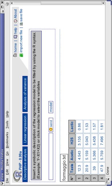
2.2.3 Analysis of variance
The graphical window of this GUI is very similar to the linear regression one; also
in this GUI, besides the data set previously loaded, there is a text area where it is
possible to input the model formula, by using the R syntax. About the data input,
the user has to input balanced data set if he wants easily interpretable results, as it
is known. Even in this GUI, if a user edits a dangerous command in the text area,
commands are not executed and an error message appears with the possibility toCHAPTER 2. USER GUIDE 24
visualize the banned command list. Actually, it is not necessary the user inputs the
model formula directly, but can choose to click on the model button that opens a
new window where it is possible to choose the response variable and the explanatory
variables among those of the loaded data set. If the explonatory variables are numeric,
the implemented code forces these variables to factors before the analysis of variance
is performed. In this window we have implemented some checks, so:
• it is not possible to choose no response variable or more than one;
• it is necessary to choose at least one explanatory variable;
• the same variable can not be chosen as response and explanatory variable at
the same time.
After the response and the explanatory variables have been chosen, this window
is closed and the main window appears slightly modified. In particular, under the
text area where the model formula is inserted, the levels of the chosen explanatory
variables are shown. Close to the model button, a new button is shown, giving the
possibility to the user to insert possible interactions in the model.
Now, the user can perform the analysis of variance with the chosen model by
clicking on the send button. Then, the output window is shown; this window contains
the following information:
• the variables involved in the model;
• the levels of each factor;
• the main descriptive statistics computed on the variables involved on the model;
• the analysis of variance table;
• the graphs of the analysis of residuals.
When a multi-way analysis of variance is performed and there is only one obser-
vation per cell, the error has a sum of squares equal to zero with a consequent lossCHAPTER 2. USER GUIDE 25
of validity of the F test. In these cases, R-php, after the analysis of variance table,
stops the running code and gives an error message explaining the problem to the user.
At this point, the user is adviced to go back to the GUI main window, by reinputing
the model formula with no interaction of the highest order. Moreover, in the output
window there are buttons to save:
• all the output in .pdf format;
• every single plot in .png format.
2.3 Examples of use of R-php point-and-click
In this section, we are going to see some examples of use for every single GUI of
R-php point-and-click developed so far. What is next it is only an indication to the
user on how it is possible to use R-php point-and-click ; if problems were to raise in
the analysis of other data sets, it is possible to report these problems to the authors.
2.3.1 Descriptive statistics
In this section the data set of the “formaggio.txt” file is used. This file contains data
related to the concentration of several chemicals in 30 samples of Cheddar cheese from
the LaTrobe Valley of Victoria, Australia and a subjective measure of taste for each
sample (Moore e McCabe, 2002, Introduction to the practice of Statistics, Freeman
and Co.). Indeed, it is known that as cheddar cheese matures, a variety of chemical
processes take place and this fact assesses the taste of the final product. In particular,
the variables taken into account are:
• Taste: subjective taste test score, obtained by combining the scores of several
tasters.
• Acetic: natural logarithm of concentration of acetic acid.
• H2S: natural logarithm of concentration of hydrogen sulfide.CHAPTER 2. USER GUIDE 26 • Lactic: concentration of lactic acid. Loaded the data set by selecting the “formaggio.txt” file from a local directory and by choosing the Yes option of Header, the obtained result is that shown in figure 2.4. By selecting the descriptive statistics GUI it is visualized the screen reported in figure 2.5. Let’s suppose we want to compute for all the 4 variables of the data set the following descriptive statistics: minimum, maximum, mean, median and variance (see fig. 2.6). At this point the requested computations are performed when the user clicks the send button. The output window has the form reported in figure 2.7. As we have said before, in the output window there is the possibility to save the analysis results in .pdf; the content of the .pdf file for this analysis is reported in appendix. 2.3.2 Linear Regression To show how it can be used the linear regression GUI of R-php point-and-click, let’s consider the same file, “formaggio.txt”, used in the previous section. Loaded the data set and chosen the linear regression GUI (see figure 2.8) we want to estimate the regression model with Taste as response and the remaining variables as explanatory. By clicking on the model button, it is shown a window where it is possible to choose the response and explanatory variables; in this case, we have to click on the cross between Taste and Response, while we select the remaining variables as explanatory (see figure 2.9). By clicking on the insert button, the beginning window appears and in the text area it is shown the chosen model formula. Now, it is sufficient to click on the send button to have the results about the chosen model (see figure 2.10). As we have said before, in the output window there is the possibility to save the analysis results in .pdf; also in this case the content of the .pdf file for this analysis is reported in appendix.
CHAPTER 2. USER GUIDE                                 27

                Figure 2.4: Import of the data set.
CHAPTER 2. USER GUIDE 28
Figure 2.5: Beginning screen of the descriptive statistics GUI.CHAPTER 2. USER GUIDE 29
Figure 2.6: Selection of the statistics of the descriptive statistics GUI.CHAPTER 2. USER GUIDE 30
Figure 2.7: Output of the descriptive statistics GUI.CHAPTER 2. USER GUIDE 31
Figure 2.8: Beginning screen of the linear regression GUI.CHAPTER 2. USER GUIDE 32
Figure 2.9: Window to select the variables.
2.3.3 Analysis of variance
About the analysis of variance we are going to see a first example of one-way analysis
of variance. Let’s consider the data set of the “capelli.txt” file. This file contains
data related to a study conducted at the University of Melbourne to indicate if there
may be a difference between the pain thresholds of blonds and brunettes (McClave
e Dietrich, 1991, Statistics, Dellen Pubblishing). In particular, men and women of
various ages were divided into four categories according to hair colour: LightBlond,
DarkBlonde, LightBrunette, DarkBrunette. The purpose of the experiment was toCHAPTER 2. USER GUIDE 33 determine whether hair colour is related to the amount of pain produced by common types of mishaps and assorted types of trauma. Each person in the experiment was given a pain threshold score based on his or her performance in a pain sensitivity test (the higher the score, the higher the person’s pain tolerance). The variables are: HairColor and Pain. First, let’s import the file as we have described previously. By choosing the analysis of variance GUI, it is showed the related window. Now, by clicking on the model button, it is shown a window that permits to the user to choose the response variable and the factors; in this case, we have to click on the cross between HairColor and Explanatory and between Pain and Response (see figure 2.11). By clicking on the insert button, we go back to the GUI beginning window that now it is slightly different. Indeed, in the text area it is shown the chosen model formula and, below, the level of the previously chosen factors (see figure 2.12). Now, it is sufficient to click on the send button to have the results about the chosen model (see figure 2.13). As we have said before, in the output window there is the possibility to save the analysis results in .pdf; also in this case the content of the .pdf file for this analysis is reported in appendix. Now, we are going to see two examples of two-way analysis of variance: the former in which we have a data set with one observation per cell and then we have to suppose a null interaction effect, the latter in which we have a balanced design with more than one observation per cell and then we have to consider the interaction effect. For the former case, we consider the “lunapiena.txt” file. In folklore, the full moon is often portrayed as something sinister, a kind of evil force possessing the power to control our behaviour. Over the centuries, many promi- nent writers and philosophers have shared this belief. The data give the admission rates to the emergency room of a Virginia mental health clinic before, during and after the 12 full moons from August 1971 to July 1972. These data are taken to see if it has grounds the popular belief that the full moon is often portrayed as something sinister (Larsen & Marx, 1986, An Introduction to Mathematical Statistics and Its Applications, 3a edizione, Prentice Hall). The
CHAPTER 2. USER GUIDE                                                                  34

variables taken into account are Admission, i.e. the daily admission rate; Month,
i.e. month of year; Moon, i.e. before, during or after the full moon. As before,
let’s import tha data set and let’s choose the analysis of variance GUI. Then, by
clicking on the model button, it is shown a window where it is possible to choose the
response variable and the factors; in this case, we have to click on the cross between
Month and Explanatory, between Moon and Explanatory and between Admission
and Response (see figure 2.14).
   At this point we return to the previous page and the add-interactions button
is shown; this button allows to add the possible interactions; in this case we do not
use this button and we go on with the analysis by clicking the send button. Then
the output window is visualized (see figure 2.15).
   As we have said before, in the output window there is the possibility to save the
analysis results in .pdf; also in this case the content of the .pdf file for this analysis
is reported in appendix.
   Let’s see, now, an example of two-way analysis of variance with an interaction ef-
fect; for this example, we use the “insulate.txt” file. This data set has three variables:
the response variable Strength, i.e. the impact strength of an insulating material,
in foot/pounds, and the explanatory variables Lot, i.e. the lot of insulating material
and Cut, i.e. the type of cut (Ostle & Malone, 1987, Statistics in Research: Basic
Concepts and Techniques for Research Workers, 4a edizione, Blackwell Pubblishing).
   As before, let’s import tha data set and let’s choose the analysis of variance GUI.
Now, by clicking on the model button, it is shown a window where it is possible to
choose the response variable and the factors; in this case, we have to click on the
cross between Cut and Explanatory, between Lot and Explanatory and between
Strength and Response (see figure 2.16).
   By clicking the insert button, we return to the previous page and the add-interactions
button is shown; this button allows to add all the possible interactions; in this case
we select the two variables to estimate their interaction effect (see figure 2.17)
   By clicking the insert button, the model is input with the interaction in the
suitable text area and by clicking the send button, the output is visualized in a new
window (see figure 2.18).
CHAPTER 2. USER GUIDE                                                                  35

   As we have said before, in the output window there is the possibility to save the
analysis results in .pdf; also in this case the content of the .pdf file for this analysis
is reported in appendix.
CHAPTER 2. USER GUIDE                                          36

           Figure 2.10: Output of the linear regression GUI.
CHAPTER 2. USER GUIDE 37
Figure 2.11: Window to select the variables.CHAPTER 2. USER GUIDE 38
Figure 2.12: Screen of the analysis of variance GUI.CHAPTER 2. USER GUIDE 39
Figure 2.13: Output of the analysis of variance GUI.CHAPTER 2. USER GUIDE 40
Figure 2.14: Window to select the variables.CHAPTER 2. USER GUIDE 41
Figure 2.15: Output of the analysis of variance GUI.CHAPTER 2. USER GUIDE 42
Figure 2.16: Window to select the variables.CHAPTER 2. USER GUIDE 43
Figure 2.17: Window to select the interactions.CHAPTER 2. USER GUIDE 44
Figure 2.18: Output of the analysis of variance GUI.APPENDIX
output R−PHP − http://r−php.homelinux.net

[1] "Taste"    "Acetic" "H2S"      "Lactic"

                          Taste

Min
[1] 0.7

Median
[1] 20.95

Mean
[1] 24.53333

Max
[1] 57.2

Variance
[1] 264.2375

                          Acetic

Min
[1] 4.477

Median
[1] 5.425

Mean
[1] 5.498033

Max
[1] 6.458

Variance
[1] 0.3259021

                          H2S

Min
[1] 2.996

                                                                     1
output R−PHP − http://r−php.homelinux.net
Median
[1] 5.329
Mean
[1] 5.941767
Max
[1] 10.199
Variance
[1] 4.523615
Lactic
Min
[1] 0.86
Median
[1] 1.45
Mean
[1] 1.442
Max
[1] 2.01
Variance
[1] 0.0921062
2output R−PHP − http://r−php.homelinux.net
[1] "Taste" "Acetic" "H2S" "Lactic"
Taste Acetic H2S Lactic
Min. : 0.70 Min. :4.477 Min. : 2.996 Min. :0.860
1st Qu.:13.55 1st Qu.:5.237 1st Qu.: 3.978 1st Qu.:1.250
Median :20.95 Median :5.425 Median : 5.329 Median :1.450
Mean :24.53 Mean :5.498 Mean : 5.942 Mean :1.442
3rd Qu.:36.70 3rd Qu.:5.883 3rd Qu.: 7.575 3rd Qu.:1.667
Max. :57.20 Max. :6.458 Max. :10.199 Max. :2.010
Taste Acetic H2S Lactic
Taste 264.237471 5.0996402 26.1288011 3.4742414
Acetic 5.099640 0.3259021 0.7503155 0.1046089
H2S 26.128801 0.7503155 4.5236150 0.4162177
Lactic 3.474241 0.1046089 0.4162177 0.0921062
Taste Acetic H2S Lactic
Taste 1.0000000 0.5495393 0.7557523 0.7042362
Acetic 0.5495393 1.0000000 0.6179559 0.6037826
H2S 0.7557523 0.6179559 1.0000000 0.6448123
Lactic 0.7042362 0.6037826 0.6448123 1.0000000
Call:
lm(formula = Taste ~ Acetic + H2S + Lactic)
Residuals:
1output R−PHP − http://r−php.homelinux.net
Min 1Q Median 3Q Max
−17.391 −6.612 −1.009 4.908 25.449
Coefficients:
Estimate Std. Error t value Pr(>|t|)
(Intercept) −28.8768 19.7354 −1.463 0.15540
Acetic 0.3277 4.4598 0.073 0.94198
H2S 3.9118 1.2484 3.133 0.00425 **
Lactic 19.6705 8.6291 2.280 0.03108 *
−−−
Signif. codes: 0 `***' 0.001 `**' 0.01 `*' 0.05 `.' 0.1 ` ' 1
Residual standard error: 10.13 on 26 degrees of freedom
Multiple R−Squared: 0.6518, Adjusted R−squared: 0.6116
F−statistic: 16.22 on 3 and 26 DF, p−value: 3.81e−06
Analysis of Variance Table
Response: Taste
Df Sum Sq Mean Sq F value Pr(>F)
Acetic 1 2314.14 2314.14 22.5481 6.528e−05 ***
H2S 1 2147.02 2147.02 20.9197 0.0001035 ***
Lactic 1 533.32 533.32 5.1964 0.0310795 *
Residuals 26 2668.41 102.63
−−−
Signif. codes: 0 `***' 0.001 `**' 0.01 `*' 0.05 `.' 0.1 ` ' 1
2output R−PHP − http://r−php.homelinux.net
3output R−PHP − http://r−php.homelinux.net
[1] "HairColour" "Pain"
> HairColour
[1] "DarkBlond" "DarkBrunette" "LightBlond" "LightBrunette"
Pain HairColour
Min. :30.00 DarkBlond :5
1st Qu.:40.00 DarkBrunette :5
Median :48.00 LightBlond :5
Mean :47.84 LightBrunette:4
3rd Qu.:56.00
Max. :71.00
Analysis of Variance Table
Response: Pain
Df Sum Sq Mean Sq F value Pr(>F)
HairColour 3 1360.73 453.58 6.7914 0.004114 **
Residuals 15 1001.80 66.79
−−−
Signif. codes: 0 `***' 0.001 `**' 0.01 `*' 0.05 `.' 0.1 ` ' 1
1output R−PHP − http://r−php.homelinux.net
2output R−PHP − http://r−php.homelinux.net
[1] "Month" "Moon" "Admission"
> Month
[1] "Apr" "Aug" "Dec" "Feb" "Jan" "Jul" "Jun" "Mar" "May" "Nov" "Oct" "Sep"
> Moon
[1] "After" "Before" "During"
Admission Month Moon
Min. : 5.000 Apr : 3 After :12
1st Qu.: 8.475 Aug : 3 Before:12
Median :12.850 Dec : 3 During:12
Mean :11.931 Feb : 3
3rd Qu.:14.000 Jan : 3
Max. :25.000 Jul : 3
(Other):18
Analysis of Variance Table
Response: Admission
Df Sum Sq Mean Sq F value Pr(>F)
Month 11 455.58 41.42 7.1285 5.076e−05 ***
Moon 2 41.51 20.76 3.5726 0.04533 *
Residuals 22 127.82 5.81
−−−
Signif. codes: 0 `***' 0.001 `**' 0.01 `*' 0.05 `.' 0.1 ` ' 1
1output R−PHP − http://r−php.homelinux.net
2You can also read