Learning to Represent and Accurately Arrange Food Items
←
→
Page content transcription
If your browser does not render page correctly, please read the page content below

Learning to Represent and Accurately
        Arrange Food Items
                     Steven Lee
                CMU-RI-TR-21-05
                     May 2021

                The Robotics Institute
             School of Computer Science
             Carnegie Mellon University
                Pittsburgh, PA 15213

                 Thesis Committee:
                Oliver Kroemer, Chair
                    Wenzhen Yuan
                    Timothy Lee

  Submitted in partial fulfillment of the requirements
   for the degree of Master of Science in Robotics.

             Copyright © 2021 Steven Lee

Abstract
    Arrangements of objects are commonplace in a myriad of everyday sce-
narios. Collages of photos at one’s home, displays at museums, and plates of
food at restaurants are just a few examples. An efficient personal robot should
be able to learn how an arrangement is constructed using only a few examples
and recreate it robustly and accurately given similar objects. Small variations,
due to differences in object sizes and minor misplacements, should also be
taken into account and adapted to in the overall arrangement. Furthermore, the
amount of error when performing the placement should be small relative to the
objects being placed. Hence, tasks where the objects can be quite small, such
as food plating, require more accuracy. However, robotic food manipulation
has its own challenges, especially when modeling the material properties of
diverse and deformable food items. To deal with these issues, we propose a
framework for learning how to produce arrangements of food items. We evalu-
ate our overall approach on a real world arrangement task that requires a robot
to plate variations of Caprese salads.
    In the first part of this thesis, we propose using a multimodal sensory ap-
proach to interacting with food that aids in learning embeddings that capture
distinguishing properties across food items. These embeddings are learned in
a self-supervised manner using a triplet loss formulation and a combination
of proprioceptive, audio, and visual data. The information encoded in these
embeddings can be advantageous for various tasks, such as determining which
food items are appropriate for a particular plating design. Additionally, we
present a rich dataset of 21 unique food items with varying slice types and
properties, which is collected autonomously using a robotic arm and an assort-
ment of sensors. We perform additional evaluations that show how this dataset
can be used to learn embeddings that can successfully increase performance in
a wide range of material and shape classification tasks by incorporating inter-
active data.
    In the second part of this thesis, we propose a data-efficient local regres-
sion model that can learn the underlying pattern of an arrangement using visual
inputs, is robust to errors, and is trained on only a few demonstrations. To re-
duce the amount of error this regression model will encounter at execution
time, a complementary neural network is trained on depth images to predict
whether a given placement will be stable and result in an accurate placement.
We demonstrate how our overall framework can be used to successfully pro-
duce arrangements of Caprese salads.
iv

Acknowledgments
    I would like to first thank my advisor, Professor Oliver Kroemer, for his
remarkable support and supervision over the two years that I have spent at
Carnegie Mellon University. Words cannot completely convey my gratitude for
the guidance, opportunities, and companionship that he has provided. I am also
grateful for the wonderful lab environment that he has formed around him. My
lab mates in IAM Lab have been extremely helpful in my research, academics,
and personal life. Amrita Sawhney has been an amazing lab mate and friend
over the last two years as we laughed and struggled through our work together.
Kevin Zhang, Mohit Sharma, Jacky Liang, Tetsuya Narita, and Alex LaGrassa
have all always been there to provide me with guidance when I’m stuck and
friendship outside of research. Pragna Mannam, Shivam Vats, and Saumya
Saxena have been kind and helpful since I’ve joined IAM Lab. Although the
last two years have been incredibly stressful at times, this environment made it
possible for me to have come this far.
    Additionally, I would like to thank the other members of my committee.
I would like to thank Professor Wenzhen Yuan for the support and generosity
she has shown to me by always making the time for aiding me when I request
it. Also, I would like to thank the last member of my committee, who is also
my lab mate, Timothy Lee for his guidance and feedback on my research, as
well as my career path. He has been exceptionally kind and helpful to me since
I have joined the IAM Lab and I’m very grateful to him for it.
    I’m also grateful for the funding received from Sony AI that enabled the
research discussed in this thesis. I would like to thank my friends for their
emotional support and companionship over the many years we have known
one another.
    Finally, I would like to thank my parents and sisters for their love and
support throughout my life. My parents sacrificed their dreams, passions, and
personal relationships to come to a foreign land and support my sisters and I so
we could live better lives than them. I don’t think I can ever properly convey
the respect and gratitude I have to them for raising me despite their struggles.
And to my five older sisters, I would to thank them for their love, kindness,
and advice over the years.
vi

Contents

1   Introduction                                                                                                              1

2   Learning Food Item Representations through Interactive Exploration                                                      3
    2.1 Introduction . . . . . . . . . . . . . . . . . . . . . . . . . . . . . .                             .   .   .   . 3
    2.2 Related Work . . . . . . . . . . . . . . . . . . . . . . . . . . . . .                               .   .   .   . 4
    2.3 Robotic Food Manipulation Dataset . . . . . . . . . . . . . . . . .                                  .   .   .   . 5
        2.3.1 Experimental Setup . . . . . . . . . . . . . . . . . . . . . .                                 .   .   .   . 5
        2.3.2 Data Collection . . . . . . . . . . . . . . . . . . . . . . . .                                .   .   .   . 7
        2.3.3 Data Processing . . . . . . . . . . . . . . . . . . . . . . . .                                .   .   .   . 9
    2.4 Learning Food Embeddings . . . . . . . . . . . . . . . . . . . . . .                                 .   .   .   . 9
    2.5 Experiments . . . . . . . . . . . . . . . . . . . . . . . . . . . . . .                              .   .   .   . 11

3   Learning to Accurately Arrange Objects                                                                                   15
    3.1 Introduction . . . . . . . . . . . . . . . . .   .   .   .   .   .   .   .   .   .   .   .   .   .   .   .   .   .   15
    3.2 Related work . . . . . . . . . . . . . . . .     .   .   .   .   .   .   .   .   .   .   .   .   .   .   .   .   .   16
    3.3 Technical approach . . . . . . . . . . . . .     .   .   .   .   .   .   .   .   .   .   .   .   .   .   .   .   .   17
        3.3.1 Learning High-level Arrangements           .   .   .   .   .   .   .   .   .   .   .   .   .   .   .   .   .   17
        3.3.2 Placing Strategies . . . . . . . . . .     .   .   .   .   .   .   .   .   .   .   .   .   .   .   .   .   .   21
        3.3.3 Data Collection . . . . . . . . . . .      .   .   .   .   .   .   .   .   .   .   .   .   .   .   .   .   .   23
    3.4 Experiments . . . . . . . . . . . . . . . . .    .   .   .   .   .   .   .   .   .   .   .   .   .   .   .   .   .   25
        3.4.1 Experimental Setup . . . . . . . . .       .   .   .   .   .   .   .   .   .   .   .   .   .   .   .   .   .   25
        3.4.2 Experimental Results . . . . . . . .       .   .   .   .   .   .   .   .   .   .   .   .   .   .   .   .   .   25

4   Conclusion                                                                                                               31

Bibliography                                                                                                                 33

                                            vii
viii
List of Figures

 2.1    Experimental setup for the robot cutting data collection . . . . . . . . . .     .   5
 2.2    Example images from experimental setup for collecting robot cutting data         .   5
 2.3    Experimental setup for the data collection involving a robot playing with
        food . . . . . . . . . . . . . . . . . . . . . . . . . . . . . . . . . . . . .   . 6
 2.4    Example images from experimental setup for collecting robot playing data         . 6
 2.5    Example images of the food items in our dataset . . . . . . . . . . . . . .      . 8
 2.6    Overview of our approach to learning embeddings from our food dataset .          . 10
 2.7    Visualization of audio PCA features from the robot playing data . . . . .        . 14
 2.8    Visualization of our learned embeddings of the robot playing audio data .        . 14

 3.1  Overview of our approach to accurately arranging objects . . . . . . . . . .           17
 3.2  Features used to train the Product of Experts model . . . . . . . . . . . . .          19
 3.3  Network architecture for our recurrent neural network arrangement predictor            20
 3.4  Training pipeline for our binary stability classifier. . . . . . . . . . . . . . .     22
 3.5  Real world gripper design . . . . . . . . . . . . . . . . . . . . . . . . . . .        22
 3.6  Experimental setup for our robot arranging setup . . . . . . . . . . . . . .           24
 3.7  Arrangement results of our Product of Experts model . . . . . . . . . . . .            26
 3.8  Effect of using different length scales for the gaussian experts . . . . . . . .       26
 3.9  Effect of samples size on our Product of Experts model . . . . . . . . . . .           27
 3.10 Real world arrangement results . . . . . . . . . . . . . . . . . . . . . . . .         28
 3.11 Images of food items used for classifying which slices are appropriate for
      an arrangement. . . . . . . . . . . . . . . . . . . . . . . . . . . . . . . . .        29
 3.12 Distance matrices between the learned embeddings of the items used for
      appropriate arrangement classification . . . . . . . . . . . . . . . . . . . .         30

                                            ix
x
List of Tables

 2.1   Results of using our learned food embeddings on different tasks . . . . . . 11
 2.2   Results of using our learned food embeddings of uncooked food on differ-
       ent tasks . . . . . . . . . . . . . . . . . . . . . . . . . . . . . . . . . . . . 12

 3.1   Results of the classifying which items should be used for an arrangement. . 29

                                           xi
xii
Chapter 1

Introduction

    Learning to accurately recreate arrangements from visual demonstrations is a process
that humans regularly undergo when learning to perform certain tasks, such as arranging
displays at department stores, decorating desks at home, or plating food at restaurants. For
robots that will be deployed in customer service or home environments, being able to easily
learn various arrangements from visual demonstrations is a valuable ability. The process for
learning arrangements typically consists of two sub-tasks: 1) Making high-level decisions
on the appearance of the arrangement, and 2) Performing the physical actions of picking
and placing the objects according to those high-level decisions.
    When making the high-level decisions for arrangements, the choice of what objects
should be used for an arrangement can drastically affect the final result. For example, decid-
ing to place a whole tomato part way through arranging a Caprese salad that only contains
slices would not look as visually appealing as using a disc-shaped tomato slice. Having
knowledge on an object’s material properties and shape can help to inform these types of
decisions. Furthermore, this information is important for robots learning to perform tasks
that involve physical interactions, since modeling object dynamics can be crucial for said
tasks. However, obtaining this information for food items can be difficult and time consum-
ing. Food items in particular can vary widely between and within food types depending on
factors such as ripeness, temperature, how they were stored, and whether they have been
cooked [1]. Humans, as a result of our prior knowledge and access to multiple forms of
sensory information, can roughly ascertain material properties of food items through in-
teracting with them. For example, one can squeeze an avocado to identify its ripeness.
Analogously, there is evidence that the ability to distinguish properties between food items
can be learned using multimodal sensor data from interactive robot exploration [2–4]. The
sensory feedback of these interactions can form the basis for learning visual representations
that are better suited to capturing the material properties of objects.
    This thesis is composed of two works. In chapter 2, we explore a method of learning
food items embeddings, in an self-supervised manner, that encodes various material proper-
ties using multiple modes of sensory information. As a means to learn these embeddings, a
unique multi-modal food interaction dataset is collected consisting of vision, audio, propri-
oceptive, and force data, which is acquired autonomously through robot interactions with a
variety of food items. The network used to learn these embeddings is trained using a triplet
loss formulation, which groups similar and dissimilar data samples based on the different

                                              1
modalities of interactive sensor data. In this manner, the robot can learn complex represen-
tations of these items autonomously without the need for subjective and time-consuming
human labels.
Once these food item representations are learned, they can be utilized to improve dif-
ferent manipulation tasks. For example, they can be used as a basis for determining what
items are appropriate for an arrangement’s appearance. However, making high-level deci-
sions on an arrangement’s appearance also require that the robot can adapt to varying object
sizes and unexpected misplacements that may occur, while only requiring a small number
of training demonstrations. Furthermore, a robot making these decisions would also need
to take into account human preferences, which is difficult since there is not an unbiased and
quantitative way to measure whether an arrangement will be appealing to humans or not.
Even if a decision making system is able to accomplish these feats, robotic placements
that lead to large and irreversible errors can still occur. Therefore, it is also essential that
the resulting placements are as accurate as possible. One could try to resolve these errors
after the placement by physically adjusting their positions, but this could lead to more
operation costs or even damage the objects. For example, this would be impractical for
tasks involving delicate and deformable objects, such as plating thin slices of food. Instead,
we can learn a method to determine when these types of errors may occur.
In chapter 3, we aim to address these issues by learning how to accurately recreate the
patterns found in arrangements in a manner that is robust and can accommodate for er-
rors in placement, while still accommodating human preferences. For making decisions on
where to place objects, we learn a local product of experts model for each placement, which
is trained using a low number of samples and can easily incorporate additional information
through weighting of the training samples and additional experts. We also train a compli-
mentary neural network to perform binary classification on whether a particular object, and
the surface it will be placed on, will lead to a misplacement when given only depth images
of the two. Rather than trying to accurately predict complex shifting behaviours using re-
gression, our approach focuses on identifying locations where the placed objects will not
shift significantly.
To demonstrate the utility of the learned food item representations, which will be dis-
cussed in chapter 2, we use them as input features to train regressors and classifiers for
different tasks and compare their performances with baseline vision-only and audio-only
approaches. For our high-level arrangement approach, which we will discuss in chapter 3,
we evaluate it on multiple different arrangements. Similarly, we evaluate our binary classi-
fication network on a variety of placements in simulation and the real world. We evaluate
our entire pipeline in the real world by constructing multiple plating arrangements of Cap-
rese salads.
2Chapter 2
Learning Food Item Representations
through Interactive Exploration
2.1 Introduction
In this chapter, we explore a self-supervised method to learning food item representa-
tions that embed various material properties and uses only visual input at test time. These
embeddings are learned from a self-procured, unique multimodal dataset consisting of au-
dio, vision, proprioceptive, and force data acquired autonomously through robot interac-
tions with a variety of food items. The neural network used to learn these embeddings is
trained using a triplet loss formulation, where groups of similar and dissimilar samples are
formed based on the different modes of the interactive sensor data. In this manner, the
robot can learn complex representations of these items autonomously without the need for
subjective and time-consuming human labels. Furthermore, we share our dataset, which
consists of 21 unique food items with varying slice types and properties, here1 . Our project
website can also be found here2 .
We demonstrate the utility of the learned representations by using them as input features
to train regressors and classifiers for different tasks and compare their performances with
baseline vision-only and audio-only approaches. Our experiments show that classifiers
and regressors that use our learned embeddings outperform the baseline approaches on
a variety of tasks, such as hardness classification, juiciness classification, and slice type
classification. These results indicate that our visual embedding network encodes additional
material property information by utilizing the different modalities, while only requiring the
robot to interact with the object at training time. The work described in this chapter was
performed in collaboration with Amrita Sawhney and Kevin Zhang in [5].
1
https://tinyurl.com/playing-with-food-dataset
2
https://sites.google.com/view/playing-with-food
32.2 Related Work
Researchers have made contributions on learning deep embeddings of objects in order
to create useful representations, which can be used on a wide range of tasks [6–8]; however,
performing the same task for food items has not been studied extensively. Sharma et al. [9]
learn a semantic embedding network, based on MaskRCNN [10], to represent the size of
food slices in order to plan a sequence of cuts. Isola et al. [11] use collections of human la-
beled images to generalize the states and transformations of objects, such as varying levels
of ripeness in fruit. Although the above works learn embeddings for food objects, both of
them focus on using solely visual inputs during both train and test time. By contrast, the
methods discussed in this chapter incorporate additional synchronized multi-modal sensory
information during the training phase of our vision-based embedding networks.
Instead of learning deep embeddings through vision, many recent works aim to learn
the dynamics models and material properties of deformable objects through simulation [12,
13]. For example, Yan et al. [14] learn latent dynamics models and visual representations
of deformable objects by manipulating them in simulation and using contrastive estimation.
Matl et al. [15] collect data on granular materials and compare the visual depth information
with simulation results in order to infer their properties. By comparison, the work discussed
in this chapter involves collecting and exploiting data from real-world robots and objects,
since representations of food that are learned through a simulation environment may not
accurately transfer to real world. This is due to the variable behaviors of food during
complex tasks, such as large plastic deformations during cutting. There are simulators that
can simulate large elasto-plastic deformation [16], but they are computationally expensive,
unavailable to the public, and have not yet shown their efficacy in this particular domain.
Other works also use multimodal sensors to better inform a robot of deformable object
properties for more sophisticated manipulation [4, 17, 18]. Erickson et al. [19] use a spe-
cialized near-infrared spectrometer and texture imaging to classify the materials of objects.
Meanwhile, Feng et al. [20] use a visual network and force data to determine the best lo-
cation to skewer a variety of food items. Tatiya et al. [21] utilize video, audio, and haptic
data as input to a network to directly categorize objects into predefined classes. Finally,
Zhang et al. [22] use forces and contact microphones to classify ingredients for obtaining
the necessary parameters to execute slicing actions. In contrast, the work discussed in this
chapter only uses images as input to our embedding network during inference time, while
still incorporating multi-modal data during training.
Finally, numerous works have focused on using interactive perception to learn about
objects in the environment [2, 23]. Yuan et al. [24, 25] use the images from GelSight [26]
sensors to create embeddings of deformable objects to determine the tactile properties of
cloth. Conversely, our work aims to learn material properties of deformable food items.
Katz et al. [27] use interactive perception to determine the location and type of articulation
on a variety of objects. Sinapov et al. [21, 28, 29] have a robot interact with objects using
vision, proprioception, and audio in order to categorize them. Chu et al. [30] utilize 2
Biotac haptic sensors on a PR2 along with 5 exploratory actions in order to learn human
labeled adjectives. In the work discussed in this chapter, we focus our exploratory data
collection on deformable food objects instead of rigid ones.
42.3 Robotic Food Manipulation Dataset
2.3.1 Experimental Setup
Our robotic food manipulation dataset was collected using a pipeline of two different
experimental setups: one setup for robotic food cutting and another for food playing. For
the food cutting setup, the robot cuts food items, using predefined cutting actions, into
specific types of slices. For the food playing setup, the robot physically interacts with these
food slices in a fixed sequence of actions. The specific types of slices and the sequence
of actions will be discussed later in this section. The multi-modal sensor data collected
during the cutting and playing data collection processes was gathered using the Franka
Emika robot control framework mentioned in [31]. The following sections describe the 2
experimental setups in further detail.
Figure 2.1: The experimental setup for collecting robot cutting data described in Sec-
tion 2.3.1. The colored boxes show the locations of the cameras and contact microphones
used to record visual and audio data respectively. Note that the contact microphones are
not clearly visible in the images shown.
Overhead Kinect Image Side RealSense Image Tong RealSense Image Knife RealSense Image
Figure 2.2: Example images from the 4 cameras used in the robotic food cutting data
collection setup described in Section 2.3.1.
Robot Cutting:
The experimental setup for the robotic cutting includes two Franka Emika Panda Arms
mounted on a Vention frame with a cutting board in the center, which is shown in Fig-
ure 2.1. One arm has its end-effector fingers replaced with a pair of mounted 8” kitchen
tongs, while the other is grasping a custom 3D printed knife attachment made of PLA.
Four cameras are used in this setup: an overhead Microsoft Azure Kinect Camera mounted
on the Vention frame, a side-view Intel Realsense D435 camera that is also mounted on
5the Vention frame, another D435 camera mounted above the wrist of the robot holding the
knife, and a third D435 camera mounted on the wrist of the robot holding the tongs. Ex-
ample images from each of the 4 cameras are shown in Figure 2.2. Additionally, there are
3 contact microphones: one mounted underneath the center of the cutting board, another
mounted on the knife attachment, and the last mounted on one of the tongs.
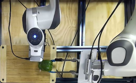
Figure 2.3: The experimental setup for collecting data as the robot plays with food. The
setup is described in Section 2.3.1. The colored boxes in the left image show the locations
of the cameras and contact microphones used to record visual and audio data respectively.
Note that the contact microphones are not clearly visible in the images shown. The right
image shows the FingerVision cameras.
Overhead Kinect Image Side RealSense Image Left FingerVision Image Right FingerVision Image
Figure 2.4: Examples images of a cut tomato from the Kinect, Realsense, and FingerVision
cameras described in Section 2.3.1.
Robot Playing:
For the robotic food playing setup, a single Franka Emika Panda Arm is mounted on
a Vention frame with a cutting board in the center, as shown in Figure 2.3. An overhead
Microsoft Azure Kinect Camera and a front-view Intel Realsense D435 camera, which is
facing the robot, are mounted to the Vention frame. A fisheye 1080P USB Camera 3 is
attached to each of the end-effector fingertips as in FingerVision [32]. It should be noted
that a laser-cut clear acrylic plate cover is used instead of a soft gel-based cover over the
camera. This acrylic plate allows for observation of the compression of the object being
3
https://www.amazon.com/180degree-Fisheye-Camera-usb-Android-Windows/dp/B00LQ854AG/
6grasped relative to fingertips. A white LED is added to the interior of the FingerVision
housing to better illuminate objects during grasping. Example images from all of these
cameras are shown in Figure 2.4. To record audio information, 2 contact microphones are
used: one is mounted underneath the center of the cutting board and the other is mounted
on the back of the Franka Panda hand. The Piezo contact microphones 4 from both cutting
and playing setups capture vibro-tactile feedback through the cutting board, end-effector
fingers, and tools. The audio from the contact microphones of both the cutting and playing
setup are captured using a Behringer UMC404HD Audio Interface 5 and synchronized with
ROS using sounddevice ros [33].
2.3.2 Data Collection
Using the robotic food cutting setup described in Section 2.3.1, we teach the robot sim-
ple cutting skills using Dynamic Movement Primitives (DMPs) [34, 35]. Ridge regression
is used to fit the DMP parameters to trajectories, which were collected using kinesthetic hu-
man demonstrations as in [22]. These DMPs are then chained into multiple slicing motions
until the food items were completely cut through.
Data was collected for 21 different food types: apples, bananas, bell peppers, bread,
carrots, celery, cheddar, cooked steak, cucumbers, jalapenos, kiwis, lemons, mozzarella,
onions, oranges, pears, potatoes, raw steak, spam, strawberries, and tomatoes. For each
of the food types, we obtained 10 different slice types. It should be noted that across all
21 food types, there are 14 different types of slices, which were created using similar skill
parameters across the food types. The skill parameters vary in slice thickness from 3mm to
50mm, angles from ±30 degrees, and slice orientation where we had normal vs. in-hand
cuts when the knife robot cut between the tongs. 14 slice types were used instead of 10
because not all slice types can be executed on every food type, especially the angled cuts,
due to the variations in size across food types. As the slices are obtained, audio, image,
and force data is collected. Figure 2.5 shows the resulting slices for each of the food types.
In total, the cutting data in our dataset consists of 210 samples of audio, visual, and force
data, one for each of the different slices.
After the different slice types have been created, they are transferred to the robotic food
playing setup to begin the remainder of the data collection process. First, one of the slices
is manually placed on the cutting board at a random position and orientation. A RGBD
image of the slice is then captured from the overhead Kinect camera and square cropped
to the cutting board’s edges. Next, the robot performs a sequence of actions, which we
refer to as the playing interactions, on the single slice. To begin these interactions, the
center of the object is manually specified and the robot then closes its fingers and pushes
down on the object until 10N of force is measured. The robot’s position and forces during
this action are recorded. Next, the robot resets to a known position, grasps the object, and
releases it from a height of 15cm. Audio from the contact microphones and videos from
the Realsense cameras are recorded during the push, grasp, and release actions. Videos
from the FingerVision cameras are only recorded during the grasp and release actions.
Additionally, the gripper width when the grasp action has finished is recorded. Finally, a
4
https://www.amazon.com/Agile-Shop-Contact-Microphone-Pickup-Guitar/dp/B07HVFTGTH/
5
https://www.amazon.com/BEHRINGER-Audio-Interface-4-Channel-UMC404HD/dp/B00QHURLHM
7Figure 2.5: Example images of the food item slices in our dataset. From left to right and top
to bottom, the images show: apple, banana, bell pepper, boiled apple, boiled bell pepper,
boiled carrot, boiled celery, boiled jalapeno, boiled pear, boiled potato, bread, carrot, celery,
cheddar, cooked steak, cucumber, jalapeno, kiwi, lemon, mozzarella, onion, orange, pear,
potato, raw steak, spam, strawberry, and tomato. Note that the boiled food items are part of
the auxilary dataset that is discussed in Section 2.5
RGBD image from the overhead Kinect camera is captured. This sequence of actions is
performed 5 times in total on each of the 10 slice types from each of the 21 food types,
meaning there are 1050 samples of audio, visual, and proprioceptive data in total for the
playing data. It should be noted that in order to capture variations in the objects’ behaviors
due to differing initial positions, orientations, and changes over time, we randomly place
the slices at the beginning of each of the 5 trials.
The full dataset is available for download here6 . The data is located in the appropriately
named folders and are sorted first by food type, then slice type, and finally trial number.
Additionally, food segmentation masks are provided in the silhouette data folder. Deep
Extreme Cut (DEXTR) [36] was used to obtain hand labeled masks of the objects in the
6
https://tinyurl.com/playing-with-food-dataset
8overhead and side view images. A PSPNet [37], pre-trained on the Ade20k [38] dataset,
is then fine-tuned using the manually labeled masks previously mentioned. This fine-tuned
network is then used to generate additional segmentation masks of the other images in the
dataset. Lastly, additional playing data is provided in the old playing data folder. However,
the slices in this dataset were all hand cut, and the data was collected using a different
experimental environment.
2.3.3 Data Processing
Features are extracted from the multi-modal data so embeddings networks can be trained.
We will discuss in more detail how these features are used for training in Section 2.4. For
the audio data, the raw audio that was recorded during the cutting and playing experi-
ments (playing audio was recorded during the release, push-down, and grasp actions), was
transformed into into Mel-frequency cepstrum coefficient (MFCC) features [39] using Li-
brosa [40]. MFCC features are used because they have been shown to effectively differ-
entiate between materials and contact events [22]. Subsequently, PCA is used to extract a
lower-dimensional representation of the cutting (Acut ) and playing (Aplay ) audio features.
Proprioceptive features (P) are formed using 3 values, which are extracted from the
robot poses and forces recorded during the push down and grasp actions. The first of the 3
values is the final z position (zf ) of the robot’s end-effector, which is recorded during the
push down action once 10N of force has been reached. zf is then used to find the change
in z position between the point of first contact and zf . We will refer to this distance value
as ∆z, which provides information on an object’s stiffness. The last value for P is the final
gripper width (wg ) recorded during the grasping action once 60N of force has been reached.
These three values (zf , ∆z, and wg ) are combined to form P.
Lastly, the slice type labels (S) and food type labels (F) for each sample are used as
features. These labels are created according to the enumerated values that identify the slice
type performed during cutting and the food type of each individual sample, respectively.
The features discussed in this section are used as metrics for differentiating between similar
and dissimilar samples. We will discuss this in further detail in Section 2.4
2.4 Learning Food Embeddings
Convolutional neural networks are trained in an unsupervised manner to output embed-
dings from images of the food items. These images are taken from the overhead Kinect
camera mentioned in Section 2.3.1. Our architecture is comprised of ResNet34 [41], which
is pre-trained on ImageNet [42] and has the last fully connected layer removed. Three ad-
ditional fully connected layers, with ReLU activation for the first two, are added to reduce
the dimensionality of the embeddings. A triplet loss [43] is used to train the network, so
similarities across food and slice types are encoded in the embeddings. The loss is given
by
XN h i
Loss = kf (xai ) − f (xpi )k22 − kf (xai ) − f (xni )k22 + α (2.1)
+
i
9where f () is the embeddding network described above, N is the number of samples, xai is
the ith triplet’s anchor sample, xpi is the ith triplet’s positive sample, xni is the ith triplet’s
negative sample, and α is the margin that is enforced between positive and negative pairs.
The different modalities of data mentioned in Section 2.3.3 are used as metrics to form
the triplets and a seperate neural network is trained using each of these metrics. More
specifically, the food class labels (F), slice type labels (S), playing audio features (Aplay ),
cutting audio features (Acut ), proprioceptive features (P), and combined audio and propri-
oceptive features (Aplay +P) are used as metrics. When combining multiple features (or
modalities), we concatenate the output embeddings that were learned from the respective
networks. The F and S values are directly used to differentiate between samples. For
example, when using F as a metric, samples of tomatoes are considered positive samples
with one another and samples of any other food type are identified as negative samples. For
the other metrics (Aplay , Acut , P , and Aplay +P), we define the n nearest samples in feature
space (using the L2 norm) as the possible positive samples in a triplet and all other samples
as the possible negative samples, where n is a hyperparameter (n = 10 was used for our
experiments). Prior to training, we identify all possible positive and negative samples for
every sample in the training dataset. At training time, triplets are randomly formed using
these positive/negative identifiers. Figure 2.6 shows an overview of our approach.
To evaluate the utility of these learned embeddings, we train multiple 3-layer multilayer
perceptron classifiers and regressors for a variety of tasks, using the learned embeddings as
inputs. These results are discussed in Section 2.5.
Positive Train
Choose Triplets
Using Features Embeddings
Anchor
Linear Triplet
ResNet Layers Loss
Negative
Test
Learned
Linear Classification/
ResNet Layers
Embedding Regression Tasks
Figure 2.6: An overview of our approach to learning embeddings from our dataset. The
different features (modalities) defined in Section 2.3.3 are used to form triplets to learn
embeddings in an unsupervised manner, which are used for supervised classification and
regression tasks (blue text).
102.5 Experiments
As described in Section 2.4, embedding networks were trained using the food class la-
bels (F), slice type labels (S), playing audio features (Aplay ), cutting audio features (Acut ),
proprioceptive features (P), and combined audio and proprioceptive features (Aplay +P) for
creating triplets. These embeddings were then used to train multiple multi-layer percep-
trons to predict the labels or values for 5 different tasks: classifying food type (21 classes),
classifying the hardness (3 human-labeled classes - hard, medium, and soft), classifying
juiciness (3 human-labeled classes - juicy, medium, dry), classifying slice type (14 differ-
ent classes based on the types of cuts the robot performed), and predicting slice width (the
width of the gripper after grasping, wg ). The loss function used for predicting the slice
width is the mean squared error, while categorical cross entropy loss [44] is used for the
other 4 classification tasks. For comparison, 2 baseline approaches are also trained on the
5 tasks. One baseline is a pre-trained ResNet34 network that is trained only using visual
data and the other baseline is a 3-layer mutli-layer perceptron that uses only Aplay as input.
We chose these baselines to see how incorporating our learned embeddings, which utilize
multiple modes of sensory information, can improve performance over methods that use
only one mode of sensory information, such as visual or audio information.
To assess the generalizability of our approach, we evaluated the hardness and juiciness
classification tasks based on leave-one-out classification, where we left an entire food class
out of the training set and evaluated the trained classifiers on this class at test time. We then
averaged the results across the 21 leave-one-out classification trials. The performance of
all the trained networks on each of the tasks are shown in Table 2.1.
As shown in Table 2.1, the purely visual baseline outperforms our embeddings in the
food type classification task. This is expected since ResNet was optimized for image clas-
Hardness Juiciness Slice Type Slice
Food Type
Accuracy Accuracy Accuracy - Width
Embeddings Accuracy - 21
- 3 classes - 3 classes 14 classes RMSE
classes (%)
(%) (%) (%) (mm)
F 92.0 40.7 36.6 12.9 10.9
S 17.1 37.0 34.9 40.5 11.8
Aplay 85.7 35.0 46.0 17.1 9.9
Acut 93.5 33.5 45.6 16.8 11.3
P 49.5 47.1 37.0 20.0 7.9
Aplay +P 83.8 36.4 40.2 21.4 9.5
ResNet 98.9 34.9 36.5 30.0 13.9
Classifier w/
Aplay as 84.4 40.8 34.0 30.1 34.4
input
Table 2.1: The table shows the baseline and multi-layer perceptron results on 5 evaluation
tasks. The baseline results are shown on the last 2 rows, while the first 6 rows show results
from the networks that used the learned embeddings, described in Section 2.4, as inputs.
The best scores are shown in bold.
11Hardness Juiciness Cooked
Embeddings
Accuracy (%) Accuracy (%) Accuracy (%)
Aplay 98.0 62.9 98.9
P 63.0 68.4 60.6
Aplay +P 99.7 70.6 99.1
ResNet 90.5 66.1 90.4
Classifier w/
Aplay as 82.1 67.4 88.8
input
Table 2.2: Results on 3 evaluation tasks for different learned embedding networks that were
trained using the auxiliary cooked vs. uncooked dataset.
sification tasks and was pre-trained on the ImageNet dataset, which contains a vast number
of labeled images. However, the ResNet baseline performs worse on the other 4 tasks, as
ImageNet did not contain prior relevant information on the physical properties of the food
items, which are important for these tasks. Additionally, ResNet was structured to differ-
entiate object classes instead of finding similarities between them. Due to this, when an
entire food class was left out of the training dataset, extrapolating the correct answer from
the limited training data becomes much more challenging. Conversely, our learned embed-
dings contained auxiliary information that encoded the similarity of slices through various
multimodal features, without ever being given explicit human labels. These results indicate
that our interactive multimodal embeddings provided the multi-layer perceptrons with a
greater ability to generalize to unseen data as compared to the supervised, non-interactive
baselines.
Additionally, the results show that the audio embeddings provide some implicit infor-
mation that can help the robot distinguish food types, which can be seen in the accuracy
difference between P and Aplay +P. It is also reasonable that the proprioceptive embed-
dings are more useful at predicting hardness and slice width as their triplets were generated
using similar information. However, absolute labels were never provided when training the
embedding networks, so the learned embeddings encoded this relevant information without
supervision. It should also be noted that in the hardness and juiciness leave-one-out classi-
fication tasks, some food types, such as tomatoes, were more difficult to classify when left
out of the training dataset than others, such as carrots. This may be due to the small size of
our diverse dataset, which has few items with similar properties.
Lastly, with respect to the slice type prediction task, poor performance was observed
across all the methods due to the inherent difficulty of the task. Since there was a high
variation in shapes and sizes between food items, the slices generated by the cutting robot
experiments greatly differed at times. Therefore, it is reasonable that only the embeddings
trained using slice type labels as a metric performed relatively well on this classification
task. Overall, the results of the evaluations indicate that our learned embeddings performed
better on relevant tasks, which supports the hypothesis that they are encoding information
on different material properties and can be advantageous for certain use cases.
12Auxiliary Study with Additional Cooked vs. Uncooked Food Data
As an addendum to the 21-food class dataset described in Section 2.3.2, an additional
dataset of boiled food classes was collected to explore and evaluate our method’s ability
to detect whether a food item is cooked or not through interactive learning. The additional
boiled food classes collected were: apples, bell peppers, carrots, celery, jalapenos, pears,
and potatoes. Each item was boiled for 10 minutes and can be seen in Figure 2.5. It should
be noted that for these additional cooked food classes, the robot did not cut the food slices
due to difficulties with grasping the objects. Instead, the slices were created manually by
a human. These boiled classes were combined with their uncooked counterparts from the
full dataset to form a smaller 14-class dataset. A subset of evaluations were conducted on
embeddings learned from this dataset. Namely, predicting hardness, juiciness, and whether
an item is cooked or not. All of these evaluations were performed as leave-one-out classi-
fication tasks. The results are shown in Table 2.2.
The auxiliary study with the boiled food dataset shows that the playing audio data is
effective at autonomously distinguishing between cooked and uncooked food items, even
with the absence of human-provided labels. This behavior is likely due to the significant
changes in material properties that occur due to boiling. The high performance of the
(Aplay + P) embeddings on the hardness, juiciness, and cooked leave-one-out classification
tasks on this smaller dataset demonstrate that our approach can generalize to new data when
a food class with similar properties was present during training. For example, the following
pairs shared similar properties: apples and pears, potatoes and carrots, bell peppers and
jalapenos).
Figure 2.7 visualizes the Aplay of the different cooked and uncooked food classes in
this dataset using the top 3 principal components. Figure 2.8 visualizes the top 3 principal
components of the learned embeddings, which were based on Aplay . The colored dots
represent uncooked items, while the thinner, colored tri-symbols represent cooked items.
As shown in the plots, there is a distinct separation between the boiled and raw foods in
the audio feature space, as well as in the learned embedding space. Within the cooked
and uncooked groupings, there are certain food types that tend to cluster together. For
example, the uncooked pear and apple cluster close together, which is reasonable given the
similarities between the two fruits. Interestingly, they remain clustered close to one another
even after they are cooked, even though there is a shift in the feature space between cooked
and uncooked.
13Figure 2.7: Visualization of the playing audio features, Aplay , in PCA space. The uncooked
items are shown as dots, while the cooked items are shown as lined tri-symbols.
Figure 2.8: Visualization of the our learned embeddings, which were learned by using the
playing audio features to choose triplets, in PCA space. The uncooked items are shown as
dots, while the cooked items are shown as lined tri-symbols.
14Chapter 3
Learning to Accurately Arrange Objects
3.1 Introduction
In this chapter, we aim to learn how to accurately recreate the patterns found in ar-
rangements in a manner that is robust and can accommodate for errors, such as misplace-
ments.Our approach consists of two sub-tasks: 1) Learning the underlying pattern of ar-
rangements in a manner that is data efficient and robust to errors, while still preserving the
fundamental shapes of the arrangements, and 2) Learning where to place objects locally
so as to minimize the placement error. Our proposed method for the first task involves
learning a local product of experts model for each placement, which is trained using a few
samples and can easily incorporate additional information through weighting of the train-
ing samples and additional experts. We also explore the use of a recurrent neural network
to perform predictions on where objects should be placed. For the second task, we train a
neural network to perform binary classification on whether a particular object will lead to a
stable placement on a specific surface given only depth images as input. Rather than trying
to accurately predict complex shifting behaviours using regression, our approach focuses
on identifying locations where the placed objects will not shift significantly.
We evaluate our proposed high-level arrangement approach on multiple arrangements
and with different sets of experts and weighting hyper-parameters. Similarly, we evaluate
our binary placement classification network on a variety of placements in simulation and
the real world. Lastly, we evaluate our entire pipeline in the real world by producing
multiple plating multiple arrangements of Caprese salads.
153.2 Related work
A significant amount of work has been performed on exploring different grasping tech-
niques and gripper designs that improve the success of grasps [45–49]. Development of
advanced grippers made specifically for food grasping tasks have also been explored [50–
53]. Conversely, the amount of work related to robotic placing and arranging is not as
extensive. Many of the works that do investigate robotic placing and arranging either only
perform placements on flat and stable surfaces, or are performed on tasks that do not re-
quire a high degree of accuracy [54–57]. Jiang et al. [56, 58] introduce different supervised
learning approaches that can be used to find stable placement locations given point clouds
of the objects and placement surface. However, these placements are performed on larger
scale tasks, such as placing objects on a bookshelf or dish rack, that do not require the
same amount of precision as the tasks we are evaluating on. Later, Jiang et al. [59, 60]
learn to incorporate human preferences into their arrangements using human context in a
3-D scene. Our approach assumes that human preferences are inherently encoded in our
training data, which is not as intensive to collect, considering we do not need to extract
point clouds, human poses, or object affordances.
Other works have looked at high-level reasoning methods for dealing with arrange-
ments. Fisher et al. [61] synthesize 3-D scenes of arrangements of furniture using a proba-
bilistic model for scenes based on Bayesian networks and Gaussian mixtures. Some work
use symbolic reasoning engines to plan complex manipulation tasks involving house keep-
ing [62–64]. Sugie et al. [65] use rule-based planning to have multiple robots push a col-
lection of tables in a room. Lozano-Perez et al. [66] use task-level planning to pick and
place rigid objects on a table. These works deal with objects on a much larger scale or
focusing on producing task-level plans and parameterized actions instead seeking specific
placement locations. Cui et al. [67] utilize probabilistic active filtering and Gaussian pro-
cesses for planning searches in cluttered environments. Moriyama et al. [68] plan object
assemblies with a dual robot arm setup. Although these tasks work on smaller scale objects,
they deal with rigid objects instead of deformable objects, such as food.
Finally, a limited number of works have also looked into robotic placement of food.
Matsuoka et al. [69] use a general adversarial imitation learning framework to learn policies
to plate tempura dishes. This work utilizes tempura ingredients, which are relatively rigid,
for their arrangements, while our work deals with plating specific patterns of deformable
objects. Jorgensen et al. [70] introduce a complex robotic pick and place system for pork
in an industrial environment. Conversely, our system is aimed towards a home or kitchen
environment and does not require a specialized robotic system, only a camera and access
to a 3-D printer.
163.3 Technical approach
In this section, we will describe our approach for reproducing the patterns in different
arrangements and the techniques used to perform accurate placements. Additionally, we
will describe the process we used to collect our training data. An overview of our overall
approach is depicted in Figure 3.1.
Train Test
Simulation Data Optimize Perform
Binary Placement Placement
Stability
Classifier
Proposed
Placement
Local
Training Patterns
Weighted Start Retrieve
PoE Model Image Inputs
Figure 3.1: An overview of our approach to placing arrangements of objects. At each time
step, a local product of experts regression model is trained on images of a specific pattern
and used to make predictions on where the next object in a sequence should be placed.
These predictions are optimized using a binary stability classifier that determines whether
a placement will be stable or not.
3.3.1 Learning High-level Arrangements
Given sequences of images of object arrangements as training data, we aim to learn the
principal pattern of the arrangements so it can be recreated in a robust and flexible manner.
More specifically, the training data consists of sequences of images that are taken each time
an object is placed. We extract the bounding box of the last object in each sequence and use
this information to train the model to predict where we should place the objects to recreate
the patterns. We evaluate 2 different types of models: One being a set of low sample local
weighted regression models that use a product of experts formulation and the other being a
recurrent neural network.
Local Weighted Product of Experts (PoE) Model
For a target arrangement that contains M objects, (M − 1) local regression models are
trained, since the model for the initial object in an arrangement is either explicitly defined
by the user or taken from the distribution of initial objects. Training data is extracted from
the images and bounding box information mentioned above. Each image and bounding
box pair across all the sequences in a training dataset is considered a training sample. We
17will describe the specific feature values extracted from these samples in more detail later
in this section. Using this data, we train a Product of experts (PoE) model [71] to perform
each of the (M − 1) predictions of where placements should be made to recreate patterns.
The mth model is given by
K
1Y
fm (x| {∆mk }) = fmk (x | ∆mk ) (3.1)
Z k=1
where Z is a normalization factor, m ∈ {1, ..., M − 1}, K is the number of experts for each
local model, and ∆mk are the k th feature values that the mth model is conditioned on. We
will elaborate on these values later in this section.
For this task, we chose a multidimensional Gaussian distribution to represent each in-
dividual expert. Thus, the mean and inverse covariance of the resulting joint distribution
for the mth model are given as
K
!
X
µm = C m Ck−1 µk (3.2)
k=1
K
X
−1
Cm = Ck−1 (3.3)
k=1
where µk and Ck are the mean and covariance of the k th expert. These values are given by
PN (i) (i) (i)
i=1 ws wt x
µk = PN (i) (i)
(3.4)
i=1 ws wt
PN (i) (i) T
i=1 ws wt x(i) − µ x(i) − µ
Ck = (i) (i) 2
(3.5)
1− N
P
i=1 (ws wt )
where N is the number of training samples used, x(i) is the ith training sample’s feature
(i) (i)
value, and ws and wt are the sample weights for the N training samples. These weights
are calculated using two distance metrics. One metric being their euclidean distance to a
(i)
reference object. ws uses this metric to weigh training samples that are spatially closer
more heavily. When training the mth model, the reference object would be the (m − 1)th
object in the current arrangement and their euclidean distance would be calculated using
the bounding box centers of each object. Note that m = 0 for the first object in an
(i)
arrangement, for which we did not train a model. The other weight, wt , uses the temporal
distance as a metric for weighing samples more heavily. The temporal distance refers to the
difference between the m value of the current model, which would be the reference value,
and of the training samples. The weights are calculated using a normal distribution
!
(i)
1 1 (xs − µs )2
ws(i) (x(i)
s |µ s , σ2 ) = √ exp − (3.6)
σs 2π 2 σs2
18(e)
ΔL
(c)
ΔL
ΔG
Figure 3.2: Features used to train the experts described in Sec. 3.3.1 for our experiments.
The orange and purple lines shows local features conditioned on the distance between the
objects’ edges and centers, respectively. Red depicts a global feature conditioned on the
distance between the centers of the placing surface and objects.
where σs is a free parameter and µs is the reference value, and xis is cartesian coordinates
(i)
of the center of ith training sample’s bounding box. The wt values are calculated in the
same manner, but σs and µs are replaced with σt and µt , respectively.
The feature values we use to train each expert can be divided into two sub-classes,
which we will refer to as local and global features. We will denote local and global features
using L and G subscripts, respectively. The global feature data, ∆G , is extracted from the
bounding information by calculating the euclidean distance between a training sample and
a fixed global reference point. This reference point is defined as the center of the placing
surface.We train one expert using ∆G .
(c) (e) (c)
For local features, we extract two types of data: ∆L and ∆L . ∆L is calculated as the
distance between the mth object’s bounding box center relative to the center of the (m−n)th
(e)
object, where both objects are in the same arrangement. Similarly, ∆L is calculated as the
distance between the mth object’s bounding box edge relative to the edge of the (m − n)th
object, where both objects are in the same arrangement. We use the edges with the lowest
(e)
x and y values when calculating ∆L . For the local features, n can range from 1 to (M − 1)
and requires that we include a separate expert for each value of n. Note that the mth model
can only contain experts where (m − n) ≥ 0. Figure 3.2 shows representations of the three
global and local features.
We can use the σs and σt values to control the importance of samples for each feature.
For example, we set σs to a large value (irrelevant) and σt to a small value (relevant) for
expert conditioned on the global feature data, ∆G . This Gaussian will tend to fit over all of
the samples whose m value is closer to the current model’s value more heavily. since it is
more likely that those samples were placed in similar locations. For the experts conditioned
on the local feature data, ∆L , we set σs to a smaller value and σt to a value that is slightly
higher than σs . We want these experts to fit over samples that have similar m values, but
that are also close in proximity.
19After the mth model is learned, we use the resulting distribution to determine the next
placement location. Cross entropy optimization is used by sampling placement locations
across the placing surface and evaluating density values for each. We propose the sample
that has the best score as the next placement location. This location is further optimized
using the methods that will later be described in 3.3.2. The process is repeated for each m.
FC:1 x 1 x 256
x0 xt xn
LSTM LSTM LSTM
ResNet-34
h0 ht hn
Linear
Layers
Figure 3.3: Network architecture for our recurrent neural network predictor. A sequence of
images is given as input and predictions are made on the bounding box of the last object,
as well as the where the next placement should be made.
Recurrent Neural Networks
Aside from the PoE approach mentioned in the previous section, we additionally ex-
plore a deep learning method using recurrent neural networks (RNN). The network is
trained in a supervised manner to predict placement locations using sequences of images
as training data. Figure 3.3 shows an overview of our network architecture. Each training
sample for this network is a single fixed length sequence of images taken after each place-
ment for a specific pattern. Note that we train separate models for different patterns. For
a single sample, we first pass each image in the sequence through ResNet-34 [41], which
has its last layer removed, and and an additional 3 linear layers to create 256 length em-
beddings. We then use these embeddings for two separate predictions. The first prediction
is obtained by passing the sequence through LSTM units to predict the placement location,
which is compared to the ground truth value since we know the bounding box of where
the placement will be made during training. As a means to improve the network’s ability
to make these predictions, we additionally make predictions on the bounding box of the
last object in the input images. We use the ResNet embeddings to make predictions on
the bounding box center coordinates and dimensions after they have been passed through
another 3 linear layers to reduce the embedding size to 4. We use the Adam optimizer [72]
during training and the loss we use is a combination of L2 errors given by
20n n
1 X 1X
(xi − x̂i )2 + (yi − ŷi )2 + (ui − ûi )2 + (vi − v̂i )2 +
Loss =
n i=1 n i=1
n
" q 2 #
1 X √ p 2 p
wi − ŵi + hi − ĥi (3.7)
n i=1
where n is the number of training samples per iteration, (xi , yi ) are the coordinates of
the predicted placement location, (x̂i , ŷi ) is the ground truth placement location, (ui , vi )
are the coordinates of the center of the bounding box around the last object, and (ûi , v̂i ) is
the ground truth bounding box center, (wi , hi ) are the bounding box dimension of the last
object, and (ŵi , ĥi ) is the ground truth bounding box dimensions.
3.3.2 Placing Strategies
Once we have a proposed placement location, we wish to make the placement as ac-
curate and reliable as possible. To accomplish this, we train a neural network to perform
binary classification on whether a given placement will be stable, meaning that a large shift
will not occur, or lead to a misplacement. Rather than trying to accurately predict complex
shifting behaviours using regression, our approach focuses on identifying locations where
the placed objects will not shift significantly. Additionally, we develop a gripper design to
improve the consistency of the grasping and placing actions.
Binary Stability Classification:
We train a convolutional neural network to perform binary classification on whether a
placement will be stable. More specifically, we are referring to whether an object’s bound-
ing box center will be within some distance, r, of the expected placement location after the
object has been released from the robot’s grippers. Note that movement along the verti-
cal y-axis is ignored, only movements parallel to the table are considered when calculating
these placement shift values that are to be compared to r. Additionally, a predefined placing
skill is used from a fixed height to make the placements more consistent.
We use the network architecture proposed in [73]. The inputs to the network are two
64x64 depth images concatenated along the 3rd dimension and the end-effector pose. The
first depth image is centered at the expected placement location, while the second depth
image is centered at the center of the object that will be placed. The second image is taken
prior to the object being grasped, but we refer to this object as the in-hand object. The
two images give information on the surface of the placement area and the in-hand object,
respectively. Additionally, we rotate the image input of the in-hand object according to
what the object’s rotation about the axis normal to the placing surface will be when being
placed.
The loss is a weighted binary cross entropy loss that is weighted batchwise. The opti-
mizer used was RMSProp [74]. We use curriculum learning [75] with a manual curriculum
to train our network. Specifically, we decrease the value of r by 0.5 cm every 500 epochs.
Figure 3.4 shows the training pipeline used for learning the weights of the binary stability
classifier.
21You can also read


