IS PGD-ADVERSARIAL TRAINING NECESSARY? AL- TERNATIVE TRAINING VIA A SOFT-QUANTIZATION NETWORK WITH NOISY-NATURAL SAMPLES ONLY - OpenReview
←
→
Page content transcription
If your browser does not render page correctly, please read the page content below

Under review as a conference paper at ICLR 2019

I S PGD-A DVERSARIAL T RAINING N ECESSARY ? A L -
TERNATIVE T RAINING VIA A S OFT-Q UANTIZATION
N ETWORK WITH N OISY-NATURAL S AMPLES O NLY
 Anonymous authors
 Paper under double-blind review

                                           A BSTRACT
         Recent work on adversarial attack and defense suggests that projected gradient
         descent (PGD) is a universal l∞ first-order attack, and PGD adversarial training
         can significantly improve network robustness against a wide range of first-order
         l∞ -bounded attacks, represented as the state-of-the-art defense method. How-
         ever, an obvious weakness of PGD adversarial training is its highly-computational
         cost in generating adversarial samples, making it computationally infeasible for
         large and high-resolution real datasets such as the ImageNet dataset. In addi-
         tion, recent work also has suggested a simple “close-form” solution to a robust
         model on MNIST. Therefore, a natural question raised is that is PGD adversar-
         ial training really necessary for robust defense? In this paper, surprisingly, we
         give a negative answer by proposing a training paradigm that is comparable to
         PGD adversarial training on several standard datasets, while only using noisy-
         natural samples. Specifically, we reformulate the min-max objective in PGD ad-
         versarial training by a minimization problem to minimize the original network
         loss plus l1 norms of its gradients evaluated on the inputs (including adversarial
         samples). The original loss can be solved by natural training; for the l1 -norm
         loss, we propose a computationally-feasible solution by embedding a differen-
         tiable soft-quantization layer after the input layer of a network. We show for-
         mally that the soft-quantization layer trained with noisy-natural samples is an
         alternative approach to minimizing the l1 -gradient norms as in PGD adversar-
         ial training. Extensive empirical evaluations on three standard datasets including
         MNIST, CIFAR-10 and ImageNet show that our proposed models are comparable
         to PGD-adversarially-trained models under PGD and BPDA attacks using both
         cross-entropy and CW∞ losses. Remarkably, our method achieves a 24X speed-
         up on MNIST while maintaining a comparable defensive ability, and for the first
         time fine-tunes a robust Imagenet model within only two days. Code for the ex-
         periments will be released on Github.

1   INTRODUCTION

Although deep neural networks (DNNs) have achieved remarkable performance on various machine-
learning tasks such as object detection and recognition (Krizhevsky et al., 2012), natural language
processing (Cho et al., 2014) and game playing (Silver et al., 2016), they also have been shown to
be vulnerable to adversarial perturbations (Szegedy et al., 2013; Biggio et al., 2013). This issue
has led to broad research on adversarial attack and defense. As representative work, Madry et al.
(2017) suggest that Project Gradient Descent (PGD) is a universal first-order attack algorithm, and
PGD adversarial training is an effective method to defend l∞ first-order attacks. This conclusion
is strengthened by Carlini et al. (2017), who experimentally demonstrated that PGD-adversarial
training provably succeeds at increasing the distortion required to construct adversarial examples by
a factor of 4.2. Furthermore, PGD adversarial training is the only method that significantly increases
network robustness among all the defenses appearing in ICLR2018 and CVPR2018 (Athalye et al.,
2018; Athalye & Carlini, 2018), thus representing as the state-of-the-art defense method.
Despite the success of PGD adversarial training, one obvious limitation is that it is too compu-
tationally expensive to generate PGD adversarial examples, and thus PGD adversarial training is

                                                  1
Under review as a conference paper at ICLR 2019

impractical/infeasible on large datasets such as the ImageNet. We observe that even on the much
smaller CIFAR-10 dataset, PGD adversarial training takes a few days, while natural training only
requires several hours on a TITAN V GPU. Moreover, recent work suggests that there exists a simple
“close-form” solution to achieve robustness against l∞ attacks (Tramèr et al., 2017). The authors
observed that on average for a MNIST image, over 80% of the pixels are in {0, 1} and only 6% are
in the range [0.5 − 0.3, 0.5 + 0.3]. Thus, adversarial perturbations are 0.3/1.0 l∞ -bounded, and
the binarized versions of natural and adversarial samples can only differ in at most 6% of the input
dimensions. By simply binarizing the inputs of a naturally trained model, a robust model with only
11.4% error under a white-box iterative FSGM attack could be achieved. All the above observa-
tions raise an important question: Is PGD adversarial training really necessary in order to learn
a robust model against l∞ attacks? In this paper, we suggest the answer is “Probably No”. To
support our conclusion, we propose an alternative training approach that only requires training with
noisy-natural samples, with an objective approximately equivalent to the min-max objective in PGD
adversarial training. Specifically, we reformulate the min-max objective of PGD adversarial training
to an alternative form, which minimizes the original network loss plus the l1 norms of its gradients
in the whole data space. The original network loss can be minimized by natural training; and we
also propose noisy natural-sample training on a soft-quantization network to achieve the l1 -norm
minimization. We show that our proposed soft-quantization layer enforces nearly zero-gradients in
most areas of the data space, and noisy natural-sample training can smooth out the remaining sharp
areas to further enhance network robustness.
Though obtaining good performance, our framework seems to cause the problem of gradient mask-
ing Papernot et al. (2017). In order to show our framework is still effective, we evaluate the frame-
work together with natural and PGD adversarial training under both white-box PGD and BPDA +
PGD∗ (Athalye et al., 2018) on three standard datasets, i.e., MNIST, CIFAR-10, and ImageNet. It
is worth noting that the other two attacks proposed in (Athalye et al., 2018), i.e., EOT and Repa-
rameterization, are not applicable to our defense since no randomization or optimization loop is
incorporated in our testing stage. Surprisingly, our proposed method is comparable to PGD ad-
versarial training in terms of defense accuracy, while achieving significant speed-ups in training
as no adversarial samples are required. Specifically, the accuracy of our model is 98.49% under
100-step PGD and 87.32% under BPDA on MNIST (l∞ perturbations of  = 0.3/1.0); when l∞
perturbations are less than 0.1/1.0, our model even surpasses PGD adversarial training under the
BPDA attack. On CIFAR-10, 20-step PGD and BPDA + PGD attacks reduce the accuracy of our
model to 78.01% and 34.43% respectively, compared to 46.62% for PGD adversarial training (l∞
perturbations of  = 8.0/255.0). To the best of our knowledge, our white-box result on CIFAR10 is
currently the second-best only behind PGD adversarial training and its variants, when considering
the attacks proposed in (Athalye et al., 2018; Athalye & Carlini, 2018). For ImageNet, 20-step PGD
attack reduces the Top 1 and Top 5 accuracies of the TensorFlow-Slim library’s public Inception v3
model to 5.974% and 10.460% (l∞ perturbations of  = 4.0/255.0). When applying our proposed
defense (computationally infeasible with PGD adversarial training), we are able to obtain 32.578%
Top 1 and 69.718% Top 5 accuracies under PGD attack, and 22.582% Top 1 and 65.576% Top 5
accuracies under BPDA attack. To our knowledge, this is currently the best white-box result on
ImageNet (50000 testing samples) under PGD and BPDA + PGD.

2     P RELIMINARIES

2.1   A DVERSARIAL SAMPLES

We focus on adversarial samples on DNNs for classification, with final layers as softmax layers.
Given an input x, the network output is represented as a vector function {Fi (x)}i , with the predicted
label ỹ = argi max Fi (x). A sample x0 is defined as an adversarial sample if argi max F (x0 ) 6= y,
where y is the ground-truth label and x0 is close to the original x under a certain distance metric.

Fast Gradient Sign Method (FGSM) Fast Gradient Sign Method (FGSM) is a single-step adver-
sarial attack proposed by Szegedy et al. (2013). FGSM performs a single step update on the original
sample x along the direction of the gradient of the loss function L(x, y; θ) w.r.t. x. The update rule
   ∗
     Backward Pass Differentiable Approximation, an effective attack that breaks 5 gradient-masking-based
defenses in ICLR2018 and CVPR2018 (Athalye et al., 2018).

                                                   2
Under review as a conference paper at ICLR 2019

can be formally expressed as
                          x0 = clip[vmin ,vmax ] {x + · sign(∇x L(x, y; θ)} ,                       (1)

where  controls the maximum l∞ perturbation of the adversarial samples; [vmin , vmax ] is the image
value range and clip[a,b] (·) function forces its input to reside in the range of [a, b].

Project Gradient Descent (PGD) Projected Gradient Descent (PGD) is the strongest iterative
variant of FGSM. In each iteration, PGD follows the update rule: x0l+1 = IIclip {FGSM(x0l )}, where
FGSM(x0l ) represents an FSGM update of x0l as in (1). The outer clip function IIclip keeps x0l+1
within a predefined perturbation range. PGD can also be interpreted as an iterative algorithm to
solve the optimization problem: maxx0 :|| x0 − x ||∞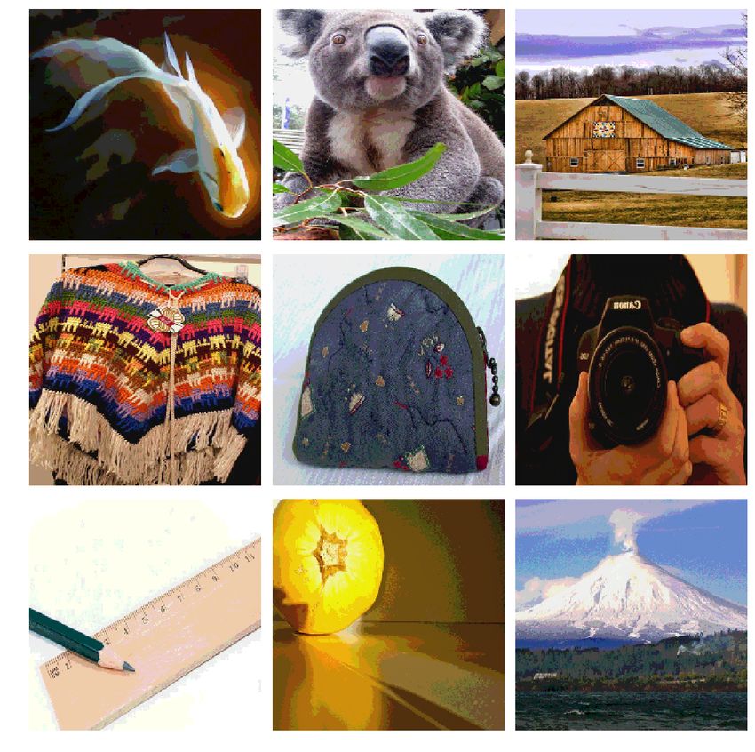
Under review as a conference paper at ICLR 2019

input into a network. Hard quantization was first proposed by Xu et al. (2017) as a feature squeezing
method to detect adversarial samples. Cai et al. (2018); Rakin et al. (2018) tried to employ hard
quantization in adversarial training to improve its defensive effectiveness against PGD. However,
since hard quantization is non-differential, the defense incorporating hard quantization will generate
infinite gradients, and thus can not be directly evaluated by gradient-based attack algorithms. Recent
work also shows that on the one hand, binarization (i.e., 1-bit hard quantization) can provide a
simple robust model against l∞ attacks on MNIST; on the other hand, a naturally-trained network
incorporating hard quantization is vulnerable to an adaptive CW-L2 attack (He et al., 2017). A
similar discretization method proposed in (Buckman et al., 2018) is also shown vulnerable to BPDA
attack (Athalye et al., 2018). Therefore, the impact of hard quantization on network robustness is
still full of uncertainty.

Soft-quantization network We propose a differentiable soft-quantization layer, whose behavior
approaches hard quantization when α is large enough but always yields finite gradients that can be
flattened by noisy training (detailed in Section 4), leading to more robust defensive ability. Specifi-
cally, a K-level soft-quantization function (layer) is defined as

                1            2k + 1        k                                    i       i+1
       S(x) = σ α(x −                ) + , where k =              min        i:
Under review as a conference paper at ICLR 2019

As shown in Figure 1, with random starts, {xt } can be considered as arbitrary samples in the data
space. As a result, the approximate objective (5) can be interpreted as simultaneously minimizing
L(x, y; θ) w.r.t. the model parameter θ and ||∇x L(x, y; θ)||1 throughout the whole data space.
The first half of this approximate objective, L(x, y; θ), can be achieved by natural/noisy training;
For the term related to 1-norm minimization, we show in the following that it can be achieved by
soft-quantization & noisy training, leading to similar defense behavior as PGD adversarial training.

Remark 1 Goodfellow et al. (2017) found that adversarial training accidentally performs gradient
masking, which can be explained by our derived gradient-masking objective (5). Actually, this
objective is intuitively correct for PGD adversarial training, in the sense that for a defense model, it
is expected not only to perform well on natural samples (the L(x, y; θ) term), but also to be robust
to adversarial samples. The later is achieved by the 1-norm term as nearly-zero ||∇x L(x, y; θ)||1
prevents generations of adversarial samples via gradient-based attack algorithms.

4.2    A N APPROXIMATE SOLUTION WITH A SOFT- QUANTIZATION NETWORK

We represent a soft-
quantization network as
      ypred = F (S(x)),     (6)
where S(·) is the soft-
quantization function and
F (·) is a standard base Figure 1: With random starts, adversarial samples could fill in the
network.    With a cross- whole data space.
entropy loss, written as
L(F (S(x)); y), the gradient w.r.t. the input x is calculated by the chain rule as
                                                ∂L(F ; y) ∂F (S) ∂S(x)
                              ∇x L(x, y; θ) =                            .                         (7)
                                                    ∂F      ∂S    ∂x
Consequently, according to Hölder’s inequality, the l1 norms are upper bounded as:
||∇x L(x, y; θ)||1 ≤ k ∂L(F ∂F
                               ;y) ∂F (S)    ∂S(x)
                                    ∂S k∞ k ∂ x k1 . Thus, to control the 1-norm ||∇x L(x, y; θ)||1 ,
it suffices to control either k ∂S(x)       ∂L(F ;y) ∂F (S)
                                 ∂ x k1 or k ∂F       ∂S k∞ , which is discussed in the following.

Controlling k ∂S(x)
                ∂ x k1 with bounded k ∂F
                                          ∂L(F ;y) ∂F (S)
                                                    ∂S k∞ We first consider the case that if
  ∂S(x)
k ∂ x k1 can be controlled small, ||∇x L(x, y; θ)||1 from our soft-quantization network defined
in Eq. 6 would also be small. According to Eq. 3,
                       ∂S(x)  α         2k + 1                  2k + 1
                             = σ(α(x −           ))(1 − σ(α(x −        )))                            (8)
                        ∂x    K          2K                      2K
                                                          i        i+1
                              where k =     min        i:
Under review as a conference paper at ICLR 2019

 Figure 2: The soft-quantization function (left) and its gradient (right) with K = 8 and α = 1000.
original samples after soft-quantization. Consequently, according to the gradient (7), the network
would not adjust for those noisy samples as long as the original samples are correctly classified.
II) For the natural samples near/in the sharp areas, it is very likely that their randomly-uniformly-
perturbed samples are still uniformly distributed around the sharp areas. In the following we show by
noisy training, gradients of the objective on these samples will also be small. For any two perturbed
samples x0 and x00 , generated from the same natural sample near/in the sharp areas, our objective
expects these two samples produce the same label y. Consequently, the cross-entropy between their
outputs can be upper bounded as
                  L(F (S(x0 )), F (S(x00 )) ≤ L(F (S(x0 )), y) + L(F (S(x00 )), y) .                (9)
The training minimizes the right hand side and thus the left side, leading to small
∇x L(x, F (S(x00 )); θ). The reason is shown below with a detailed proof given in Appendix A:
        L(F (S(x0 )), F (S(x00 ))) = L(F (S(x00 )), F (S(x00 ))) + {L(F (S(x0 )), F (S(x00 )))
                                               I x0
                       00          00
          − L(F (S(x )), F (S(x )))} ≥ 0 +           ∇x L(x, F (S(x00 )); θ) · d x .               (10)
                                                   x00

Remark 2 Using noisy samples is similar to stability training (Zheng et al., 2016), except that we
do not include the additional KL-divergence between the network outputs of natural samples and
their noisy samples in the objective. We adopt this simply because of its lower computational cost.

4.3   D ISCUSSION ON THE CHOICE OF SOFT- QUANTIZATION PARAMETER

A soft-quantization layer has two hyper-parameters as shown in Eq. 3, i.e., α and level K. Parameter
α controls the sharpness of quantization and the width of each sharp area. In the extreme case of
α = +∞, the soft-quantization function reduces to hard quantization, yielding infinite gradients
in a subspace of measure 0. In this case, sharp areas are small, but the infinite gradients would
cause training instability. Therefore, in practice, an appropriate α should be selected. In addition,
a K-level quantization would induce K n sharp areas in the whole space, where n is the dimension
of x. Thus, a small but appropriate K should be chosen, as a large K would increase the sharpness
intensity while a too small K would deteriorate the input too much. For MNIST, a good setting is to
set K = 1, equivalent to binarization if α = +∞. For CIFAR-10, a good setting we found is to set
K = 2, and for ImageNet, our setting is K = 8. More details are provided in the Appendix.

5     E XPERIMENTS
We conduct extensive experiments to compare our defense framework with the state-of-the-art de-
fense, i.e., PGD adversarial training, on three standard datasets: MNIST, CIAFR-10 and ImageNet.
For the first time, we successfully train a defense model on the largest ImageNet dataset, which
is computationally too expensive for PGD adversarial training. We detail our experiments mainly
under two white-box settings.

Adversarial setting We consider two white-box settings where the adversaries have full access to
networks including their parameters. In the first setting, the noisily-trained soft-quantization network
is directly evaluated by PGD, i.e., adversarial samples are directly crafted from the soft-quantization
network by the PGD algorithm. In the second setting, due to the gradient masking (vanishing) effect
caused by our soft-quantization layer, we evaluate our model against the BPDA adversary proposed
in (Athalye et al., 2018), which breaks many recent gradient-masking-based defenses including 5
white-box defenses in ICLR2018 and CVPR2018 (Athalye et al., 2018; Athalye & Carlini, 2018).
Since in our proposed network F (S(x)), S(x) is the major cause of gradient masking, according to
(Athalye et al., 2018), we substitute S(x) with x and craft adversarial samples from F (x) using PGD

                                                   6
Under review as a conference paper at ICLR 2019

Figure 3: MNIST: classification accuracy of Natural, PGD-Defense, SQ, and NSQ under 100-
step PGD (first two columns) and BPDA attacks (last two columns) on the cross-entropy loss (odd
columns) and CW∞ loss (even columns).

on cross-entropy and CW∞ losses† . It is worth noting that the Expectation over Transformation
(EOT) and Reparameterization methods proposed in (Athalye et al., 2018) are not applicable to our
model, since we do not incorporate any randomization or optimization loop in the testing stage of
our model. Besides, for Natural and PGD adversarial training, the BPDA adversary is equivalent to
PGD attack, since there is no transformation g(·)‡ that mainly causes gradient masking in Natural
or PGD adversarial training (Athalye et al., 2018). In the following, we denote a naturally-trained
network as Natural, a PGD adversarially-trained model as PGD-Defense, a Naturally-trained Soft-
Quantization network as SQ, and a Noisily-trained Soft-Quantization network as NSQ.

MNIST In this experiment, we adopt a basic network as a convolutional neural network (CNN)
with two convolutional layers and a fully connected layer. A soft-quantization layer with K = 1
and α = 1000 is embedded as a soft-quantization network, which is trained with natural samples
injected with random uniform noise in the range of [−0.3/1.0, 0.3/1.0]. The naturally-trained model
and PGD adversarially-trained model for comparisons are adopted from MIT MadryLab§ . The
classification accuracies of the three methods under 100-step PGD and BPDA + PGD are shown in
Figure 3. With only PGD attacks, SQ and NSQ even slightly outperform PGD-Defense. Specifically,
the accuracy of our NSQ remains 98.49%, nearly 6% higher than the accuracy of PGD-Defense (with
l∞ perturbations of  = 0.3/1.0). When considering gradient masking, the classification accuracy
of NSQ remains 87.32%, only 5% lower than the accuracy of PGD-Defense. Interestingly, when the
l∞ perturbations are smaller than 0.1/1.0, NSQ even outperforms PGD-Defense under the BPDA
attack. Notably, to achieve such robustness against PGD and BPDA adversaries, our NSQ only takes
about 5 mins with a TITAN V GPU for a 50000-iteration training procedure with minibatch size 100,
while PGD-adversarial training takes about 2 hours, achieving a 24X speed-up.

CIFAR-10 We use a residual CNN consisting of five residual units and a fully connected layer as
the basic network. A soft-quantization network with K = 2 and α = 100 × 255 ¶ soft-quantization
layer is adopted, which is trained by natural samples injected with [−16.0/255.0, 16.0/255.0] ran-
dom uniform noise. Again, the naturally-trained model and PGD adversarially-trained model are
adopted from MadryLab k . The accuracies of all the models under 20-step PGD and BPDA are
shown in Figure 4. Specifically, 20-step PGD and BPDA attacks reduce the accuracy of NSQ to
78.01% and 34.43% respectively (with l∞ perturbations of  = 8.0/255.0). To the best of our
knowledge, this is the second-best white-box result on CIFAR-10 (only worse than PGD adversarial
training), considering all defenses proposed in ICLR2018 and CVPR2018. In terms of the running
time, our NSQ only takes 9 hours training for 80000 iterations with minibatch size set to 128, while
PGD adversarial training takes more than 3 days on a TITAN V GPU.

ImageNet For the large ImageNet dataset, we adopt the widely-used Inception v3 model as the
basic network (Szegedy et al., 2016). A soft-quantization network with K = 8 and α = 10000 is
used, which is fine-tuned from a pre-trained Inception v3 model ∗∗ with noisy natural samples of
   †
     i.e., Logit-Space Projected Gradient Ascent (LS-PGA)
   ‡
     For our model, g(·) is the soft-quantization layer S(·).
   §
     https://github.com/MadryLab/mnist_challenge
   ¶
     In the implementation with a pixel-value range of [0, 255], α is set to 100. This corresponds to α =
100 × 255 in (3) if the pixel values are normalized to [0, 1].
   k
     https://github.com/MadryLab/cifar10_challenge
  ∗∗
     https://github.com/tensorflow/models/tree/master/research/slim

                                                   7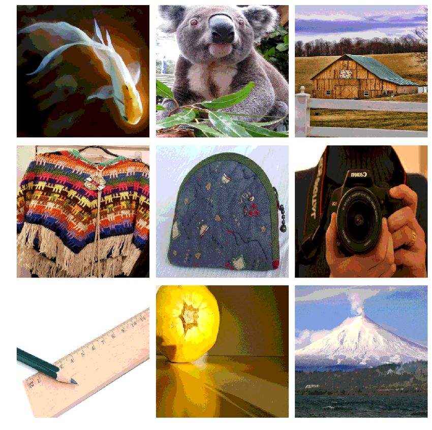
Under review as a conference paper at ICLR 2019

Figure 4: CIFAR-10: classification accuracy of Natural, PGD-Defense, SQ, and NSQ under 20-step
PGD and BPDA + PGD.

[−8.0/255.0 × 2.0, 8.0/255.0 × 2.0] random uniform noise (All the images are normalized to [-1.0,
1.0] in the preprocessing stage). Fine-tuning such a model takes less than 2 days on a TITAN GPU.
Code for implementing PGD attack is adopted from (Kannan et al., 2018) †† . To our knowledge,
there are no public PGD adversarial-trained models except only a few one-step adversarial trained
models for this large and high-resolution dataset (Kurakin et al., 2016; Tramèr et al., 2017) due
to computational infeasibility. Specifically, we observe that a single run of 10-step PGD on the
ImageNet testing dataset needs about 2 hours on a TITAN GPU. Since MadryLab’s secret CIFAR-10
model uses 128×70000 adversarial samples for training, and PGD adversarial training on ImageNet
should need at least 100 times more due to its high resolution and large data size, thus an initial
estimation of the time for PGD adversarial training on ImageNet is over 1500 days on one TITAN
GPU. As a result, we were not able to run the PGD adversarial trained model for comparison. Our
defense results are shown in Table 1, which suggest that with little sacrifice of the accuracy compared
to natural training on the clean images (no perturbation), our model obtains significant defense
accuracies under 4-pixel perturbation white-box PGD and BPDA attacks (enhance the Inception v3
model by 17% top-1 and 55% top-5 accuracies).

6   D ISCUSSION AND C ONCLUSION
Discussion Similar to PGD                                        Natural               NSQ
adversarial training, our de-              Attack
                                                            top1         top5     top1       top5
fense method only focuses on               0/255         77.978% 93.944% 73.438% 91.106%
first-order l∞ attacks. Both         4/255 20-step PGD    5.974% 10.460% 32.578% 69.718%
PGD adversarial training and        4/255 20-step BPDA       −            −     22.582% 65.576%
our method seem to be vul-
                                  Table 1: ImageNet: classification accuracies of the original Incep-
nerable to adversarial sam-
                                  tion v3 model (Natural), and the fine-tuned NSQ under 20-step PGD
ples with large l∞ perturba-
                                  and BPDA on the cross-entropy loss.
tions such as CW-L2 (Carlini
& Wagner, 2017) and EAD (Sharma & Chen, 2018). It seems that our method is still not very opti-
mal in terms of defense accuracy, leaving rooms for improvements in two directions: I) The current
defense layer is a simple soft-quantization layer. Smarter design of similar defense layers based on
the pixel-value statistics might lead to more robust defensive networks. II) Only noisy-natural sam-
ples are used to train the soft-quantization networks. A straightforward yet efficient way to improve
the network robustness is to incorporate FSGM adversarial samples in the training stage, whose
generation cost is much cheaper than that of PGD adversarial samples.

Conclusion We avoid the adversarial-sample generation in PGD adversarial training by proposing
an alternative training scheme with only noisy-natural samples. We achieve the goal by reformulat-
ing the min-max objective of adversarial training as approximately minimizing the original network
loss plus additional l1 norms of gradients in the whole data space. To alternatively achieve this
objective, we embed a soft-quantization layer into a basic network such that it yields zero-gradients
in most areas of the data space, and train the soft-quantization network with noisy natural-samples
to flatten the remaining sharp-gradient areas. Due to the gradient masking effect caused by our ap-
proach, we evaluate our model against white-box PGD and BPDA + PGD. Extensive evaluations
demonstrate that our training paradigm is comparable to PGD adversarial training in most cases
while obtaining significant speed-ups, indicating the possibility of learning a robust model with
much less effort using only noisy-natural samples.
  ††
     https://github.com/tensorflow/models/tree/master/research/adversarial_
logit_pairing

                                                  8
Under review as a conference paper at ICLR 2019

R EFERENCES
Anish Athalye and Nicholas Carlini. On the robustness of the cvpr 2018 white-box adversarial
  example defenses. arXiv preprint arXiv:1804.03286, 2018.
Anish Athalye, Nicholas Carlini, and David Wagner. Obfuscated gradients give a false sense of
  security: Circumventing defenses to adversarial examples. arXiv preprint arXiv:1802.00420,
  2018.
Battista Biggio, Igino Corona, Davide Maiorca, Blaine Nelson, Nedim Šrndić, Pavel Laskov, Gior-
  gio Giacinto, and Fabio Roli. Evasion attacks against machine learning at test time. In Joint
  European conference on machine learning and knowledge discovery in databases, pp. 387–402.
  Springer, 2013.
Jacob Buckman, Aurko Roy, Colin Raffel, and Ian Goodfellow. Thermometer encoding: One hot
  way to resist adversarial examples. 2018.
Qi-Zhi Cai, Min Du, Chang Liu, and Dawn Song. Curriculum adversarial training. arXiv preprint
  arXiv:1805.04807, 2018.
Nicholas Carlini and David Wagner. Towards evaluating the robustness of neural networks. In
  Security and Privacy (SP), 2017 IEEE Symposium on, pp. 39–57. IEEE, 2017.
Nicholas Carlini, Guy Katz, Clark Barrett, and David L. Dill. Ground-truth adversarial examples.
  CoRR, abs/1709.10207, 2017. URL http://arxiv.org/abs/1709.10207.
Kyunghyun Cho, Bart Van Merriënboer, Caglar Gulcehre, Dzmitry Bahdanau, Fethi Bougares, Hol-
  ger Schwenk, and Yoshua Bengio. Learning phrase representations using rnn encoder-decoder
  for statistical machine translation. arXiv preprint arXiv:1406.1078, 2014.
Guneet S Dhillon, Kamyar Azizzadenesheli, Zachary C Lipton, Jeremy Bernstein, Jean Kossaifi,
  Aran Khanna, and Anima Anandkumar. Stochastic activation pruning for robust adversarial de-
  fense. arXiv preprint arXiv:1803.01442, 2018.
Ian Goodfellow, Nicolas Parpernot, Sandy Huang, Yan Duan, Pieter Abbeel, and Jack Clark.
  Attacking machine learning with adversarial examples. https://blog.openai.com/
  adversarial-example-research/, 2017.
Ian J Goodfellow, Jonathon Shlens, and Christian Szegedy. Explaining and harnessing adversarial
  examples. arXiv preprint arXiv:1412.6572, 2014.
Chuan Guo, Mayank Rana, Moustapha Cisse, and Laurens van der Maaten. Countering adversarial
  images using input transformations. arXiv preprint arXiv:1711.00117, 2017.
Warren He, James Wei, Xinyun Chen, Nicholas Carlini, and Dawn Song. Adversarial example
 defenses: Ensembles of weak defenses are not strong. arXiv preprint arXiv:1706.04701, 2017.
Harini Kannan, Alexey Kurakin, and Ian Goodfellow. Adversarial logit pairing. arXiv preprint
  arXiv:1803.06373, 2018.
Alex Krizhevsky, Ilya Sutskever, and Geoffrey E Hinton. Imagenet classification with deep convo-
  lutional neural networks. In Advances in neural information processing systems, pp. 1097–1105,
  2012.
Alexey Kurakin, Ian Goodfellow, and Samy Bengio. Adversarial machine learning at scale. arXiv
  preprint arXiv:1611.01236, 2016.
Xingjun Ma, Bo Li, Yisen Wang, Sarah M Erfani, Sudanthi Wijewickrema, Michael E Houle, Grant
  Schoenebeck, Dawn Song, and James Bailey. Characterizing adversarial subspaces using local
  intrinsic dimensionality. arXiv preprint arXiv:1801.02613, 2018.
Aleksander Madry, Aleksandar Makelov, Ludwig Schmidt, Dimitris Tsipras, and Adrian Vladu.
  Towards deep learning models resistant to adversarial attacks. arXiv preprint arXiv:1706.06083,
  2017.

                                               9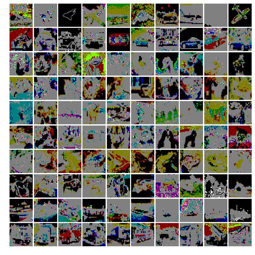
Under review as a conference paper at ICLR 2019

Taesik Na, Jong Hwan Ko, and Saibal Mukhopadhyay. Cascade adversarial machine learning regu-
  larized with a unified embedding. arXiv preprint arXiv:1708.02582, 2017.
Nicolas Papernot, Patrick McDaniel, Ian Goodfellow, Somesh Jha, Z Berkay Celik, and Ananthram
  Swami. Practical black-box attacks against machine learning. In Proceedings of the 2017 ACM
  on Asia Conference on Computer and Communications Security, pp. 506–519. ACM, 2017.
Adnan Siraj Rakin, Jinfeng Yi, Boqing Gong, and Deliang Fan. Defend deep neural networks
  against adversarial examples via fixed anddynamic quantized activation functions. arXiv preprint
  arXiv:1807.06714, 2018.
Pouya Samangouei, Maya Kabkab, and Rama Chellappa. Defense-gan: Protecting classifiers against
  adversarial attacks using generative models. arXiv preprint arXiv:1805.06605, 2018.
Yash Sharma and Pin-Yu Chen. Attacking the madry defense model with l 1-based adversarial
  examples. In Proc. of AAAI, 2018.
David Silver, Aja Huang, Chris J Maddison, Arthur Guez, Laurent Sifre, George Van Den Driessche,
  Julian Schrittwieser, Ioannis Antonoglou, Veda Panneershelvam, Marc Lanctot, et al. Mastering
  the game of go with deep neural networks and tree search. nature, 529(7587):484–489, 2016.
Yang Song, Taesup Kim, Sebastian Nowozin, Stefano Ermon, and Nate Kushman. Pixeldefend:
  Leveraging generative models to understand and defend against adversarial examples. arXiv
  preprint arXiv:1710.10766, 2017.
Christian Szegedy, Wojciech Zaremba, Ilya Sutskever, Joan Bruna, Dumitru Erhan, Ian Goodfellow,
  and Rob Fergus. Intriguing properties of neural networks. arXiv preprint arXiv:1312.6199, 2013.
Christian Szegedy, Vincent Vanhoucke, Sergey Ioffe, Jon Shlens, and Zbigniew Wojna. Rethink-
  ing the inception architecture for computer vision. In Proceedings of the IEEE conference on
  computer vision and pattern recognition, pp. 2818–2826, 2016.
Florian Tramèr, Alexey Kurakin, Nicolas Papernot, Ian Goodfellow, Dan Boneh, and Patrick Mc-
  Daniel. Ensemble adversarial training: Attacks and defenses. arXiv preprint arXiv:1705.07204,
  2017.
Cihang Xie, Jianyu Wang, Zhishuai Zhang, Zhou Ren, and Alan Yuille. Mitigating adversarial
  effects through randomization. arXiv preprint arXiv:1711.01991, 2017.
Weilin Xu, David Evans, and Yanjun Qi. Feature squeezing: Detecting adversarial examples in deep
 neural networks. arXiv preprint arXiv:1704.01155, 2017.
Stephan Zheng, Yang Song, Thomas Leung, and Ian Goodfellow. Improving the robustness of deep
  neural networks via stability training. In Proceedings of the ieee conference on computer vision
  and pattern recognition, pp. 4480–4488, 2016.
Tianhang Zheng, Changyou Chen, and Kui Ren. Distributionally adversarial attack. arXiv preprint
  arXiv:1808.05537, 2018.

                                               10
Under review as a conference paper at ICLR 2019
A P ROOF FOR E QUATION 10
We divide the cross-entropy between F (S(x0 )) and F (S(x00 )) into two terms by adding and sub-
tracting L(F (S(x00 )), F (S(x00 ))) as
L(F (S(x0 )), F (S(x00 ))) =L(F (S(x00 )), F (S(x00 )))+
{L(F (S(x0 )), F (S(x00 ))) − L(F (S(x00 )), F (S(x00 )))}. (11)
The first term is lower-bounded by 0 since
n
X
00 00
L(F (S(x )), F (S(x ))) = − Fi (S(x00 )) log Fi (S(x00 )) ≥ 0. (12)
i=1
because 0 ≤ Fi (S(x00 )) ≤ 1 .
Since F (S(x)) is the output of our soft-quantization network given input as x,
L(F (S(x0 )), F (S(x00 ))) is exactly L(x0 , F (S(x00 )); θ). Therefore, the second term can be
rewritten as
I x0
0 00 00 00
L(x , F (S(x )); θ) − L(x , F (S(x )); θ) = ∇x L(x, F (S(x00 )); θ) · d x (13)
x00
B PARAMETER STUDY ON CIFAR-10
In this section, we study the impacts of two major hyperparameters in our framework, i.e., K and α,
on the robustness of NSQ against the BPDA adversary. Because I) MNIST dataset is too peculiar
in terms of its simple binarization (i.e., K = 1 and α = +∞) solution for defense as discussed
in section 2.2 (Tramèr et al., 2017); II) it is computationally infeasible for extensive evaluations on
ImageNet, we therefore only conduct experiments on CIFAR-10 for parameter study. We plot the
classification accuracies of NSQs with different K and α in Fig. 6 and 7. As we can see, K mainly
affects the robustness of NSQ against white-box adversaries. Specifically, increasing K will enhance
the clarity of the soft-quantized images as shown in Appendix C and thus increase the classification
accuracy on clean images, but simultaneously induce more sharp areas, and therefore deteriorate
network robustness. We also observe that increasing α from 100 × 255 to 10000 × 255 will also
slightly degrade the robustness of NSQ, which can serve as weak evidence for the proposition that
the infinite gradients caused by hard quantization might lead to training instability. Considering all
of the above, K = 4 and α = 100 × 255 is a good choice for NSQ.
Figure 5: CIFAR-10: classification accuracy of different K-level soft-quantization networks under
20-step BPDA + PGD on cross-entropy and CW∞ loss (α = 1 × 255).
11Under review as a conference paper at ICLR 2019
Figure 6: CIFAR-10: classification accuracy of different K-level soft-quantization networks under
20-step BPDA + PGD on cross-entropy and CW∞ loss (α = 100 × 255).
Figure 7: CIFAR-10: classification accuracy of different K-level soft-quantization networks under
20-step BPDA + PGD on cross-entropy and CW∞ loss (α = 10000 × 255).
C VISUALIZATION OF SOFT- QUANTIZED IMAGES
The images soft-quantized by our proposed soft-quantization layer with different K and α are vi-
sualized in Fig. 8, 9, 10, 11, 12, 13 and 14. As we can see, soft-quantization with appropriate K
and α rectifies redundant information that leaves more space for an adversary to search, but retains
the sketch information that is useful for classification. As K increases, the soft-quantized images
look more like the original images, then the soft-quantization network will be more similar to the
basic network and thus more vulnerable to white-box adversaries. Hence, a small K is preferred.
However, if K is too small, especially for datasets of large diversity like ImageNet, the remaining
information after soft-quantization will be too limited for the classification task, thus the accuracy of
NSQ on both clean and adversarial samples will decrease. Therefore, in practice, selecting a small
but appropriate K is crucial to establishing and training a successful NSQ.
12Under review as a conference paper at ICLR 2019
Figure 8: MNIST: soft-quantization level K = 1. From left to right, up to down: original images,
α = 10, α = 1000, α = 100000
13Under review as a conference paper at ICLR 2019
Figure 9: CIFAR-10: soft-quantization level K = 2. From left to right, up to down: original images,
α = 1 × 255, α = 100 × 255, α = 10000 × 255
14Under review as a conference paper at ICLR 2019
Figure 10: CIFAR-10: soft-quantization level K = 4. From left to right, up to down: original
images, α = 1 × 255, α = 100 × 255, α = 10000 × 255
15Under review as a conference paper at ICLR 2019
Figure 11: CIFAR-10: soft-quantization level K = 16. From left to right, up to down: original
images, α = 1 × 255, α = 100 × 255, α = 10000 × 255
16Under review as a conference paper at ICLR 2019
Figure 12: ImageNet: from left to right, from up to down: original images, K = 4 α = 1, K = 4
α = 10000, K = 4 α = 1000000
17Under review as a conference paper at ICLR 2019
Figure 13: ImageNet: from left to right, from up to down: original images, K = 8 α = 1, K = 8
α = 10000, K = 8 α = 1000000
18Under review as a conference paper at ICLR 2019
Figure 14: ImageNet: from left to right, from up to down: original images, K = 16 α = 1, K = 16
α = 10000, K = 16 α = 1000000
19You can also read