International Journal of Psychophysiology
←
→
Page content transcription
If your browser does not render page correctly, please read the page content below
International Journal of Psychophysiology 162 (2021) 145–156
Contents lists available at ScienceDirect
International Journal of Psychophysiology
journal homepage: www.elsevier.com/locate/ijpsycho
Using multilevel models for the analysis of event-related potentials☆
Hannah I. Volpert-Esmond a, *, Elizabeth Page-Gould b, Bruce D. Bartholow c
a
Department of Psychology, University of Texas at El Paso, El Paso, TX 79968, USA
b
Department of Psychology, University of Toronto, Toronto, ON M5S, Canada
c
Department of Psychological Sciences, University of Missouri, Columbia, MO 65211, USA
A R T I C L E I N F O A B S T R A C T
Keywords: Multilevel modeling (MLM) is becoming increasingly accessible and popular in the analysis of event-related
Event-related potentials potentials (ERPs). In this article, we review the benefits of MLM for analyzing psychophysiological data,
Multilevel modeling which often contains repeated observations within participants, and introduce some of the decision-making
points in the analytic process, including how to set up the data set, specify the model, conduct hypothesis
tests, and visualize the model estimates. We highlight how the use of MLM can extend the types of theoretical
questions that can be answered using ERPs, including investigations of how ERPs vary meaningfully across trials
within a testing session. We also address reporting practices and provide tools to calculate effect sizes and
simulate power curves. Ultimately, we hope this review contributes to emerging best practices for the use of MLM
with psychophysiological data.
Psychophysiologists have long recognized that the multivariate and modeling, mixed effects modeling, and mixed effect regression—that
densely repeated-measures nature of their data call for special ap has emerged for analyzing traditionally quantified ERP components.
proaches to data analysis (e.g., Games, 1976; Keselman and Rogan, MLM is appropriate for any data that is structured such that obser
1980; Vasey and Thayer, 1987; Wilson, 1967). Over the past half- vations are recorded within naturally occurring groups. In the realm of
century most researchers have continued to use traditional approaches ERPs, multiple observations are grouped within individuals. A number
for analysis of psychophysiological data, including the use of repeated of previous articles have advocated for the use of MLM with psycho
measures ANOVA to test differences in mean amplitude or latency of physiological data, including ERPs (see Bagiella et al., 2000; Boisgontier
traditionally quantified event-related potential (ERP) components (see and Cheval, 2016; Goedert et al., 2013; Kristjansson et al., 2007; Krueger
Jennings and Allen, 2017; Luck, 2014). In the early years of the field, and Tian, 2004; Page-Gould, 2017; Tibon and Levy, 2015; Tremblay and
this practice was likely driven by the lack of available alternatives or Newman, 2015; Volpert-Esmond et al., 2018; Vossen et al., 2011). The
feasible means to carry them out. However, since statistical software purpose of this article is to provide a gentle orientation to psycho
packages for conducting complex data analyses—and desktop-type physiologists who are interested in learning more about how to apply
computers with which to run them—became available in the early MLMs to their ERP data, and to provide suggestions for best practices to
1980s, new analytic approaches have been developed that require more increase the reproducibility of these analyses and orient researchers to
intensive computational resources for fitting models, including sophis available resources to make the best analytical choices.
ticated approaches that do not rely on quantifying a particular ERP
component at a single moment in time (e.g., Kiebel and Friston, 2004; 1. Description of MLM and its advantages
Litvak et al., 2011; Pernet et al., 2011a). However, it is beyond the scope
of this article to describe all data analytic advancements for ERPs. Multilevel modeling is an extension of the General Linear Model
Instead, we focus on one popular approach—multilevel modeling (GLM) that estimates both fixed effects, as the GLM does, and random
(MLM), alternatively called hierarchical linear modeling, mixed linear effects. Fixed effects refer to effects that are expected to generalize
☆
HVE’s contribution was supported by the National Institute on Minority Health and Health Disparities (F31 MD012751). EPG’s contribution was supported by
Canada Research Chairs (CRC 152583), the Social Sciences and Humanities Research Council of Canada (Insight Grant 140649), and the Ontario Ministry of Research
and Innovation (Early Research Award 152655). BDB’s contribution was supported by the National Institute on Alcohol Abuse and Alcoholism (R01 AA025451).
* Corresponding author.
E-mail address: hivolpertes@utep.edu (H.I. Volpert-Esmond).
https://doi.org/10.1016/j.ijpsycho.2021.02.006
Received 28 August 2020; Received in revised form 1 February 2021; Accepted 3 February 2021
Available online 15 February 2021
0167-8760/© 2021 Elsevier B.V. All rights reserved.
H.I. Volpert-Esmond et al. International Journal of Psychophysiology 162 (2021) 145–156
across the population and include the estimated effects of the specified psychophysiological studies often violate core assumptions underlying
predictor or independent variables (IV) on the outcome or dependent the use of rANOVA, especially the assumption of sphericity (i.e., that the
variable (DV). Fixed effects estimated with MLM, including betas, de variance of all pairwise differences between repeated measurements is
grees of freedom, and associated p-values, are interpreted in a similar constant). As noted by numerous researchers tackling this issue (e.g.,
way as fixed effects estimated within a GLM. Unique to the MLM relative Blair and Karniski, 1993; Jennings and Wood, 1976; Keselman and
to the GLM are the random effects, which allow researchers to specify Rogan, 1980; Vasey and Thayer, 1987), the assumption of sphericity is
natural grouping variables (or “random factors”) in the data that result unrealistic when applied to psychophysiological data. Other solutions
in non-independence of observations. In the case of ERP data, random have been proposed within the context of rANOVA, including well-
factors will likely include participants and channels; however, other known adjustments to the degrees of freedom of a test—and therefore
random factors are possible, including items or the stimuli used to elicit the observed p-value—based on the degree of non-sphericity it in
the ERP signal. The intercept of the random factor can be allowed to be troduces (e.g., Greenhouse and Geisser, 1959; Huynh and Feldt, 1970,
random, meaning that a unique intercept will be estimated for each unit 1980) and multivariate tests such as Hoteling’s T2 test (Mardia, 1975).
of that random factor (e.g., if participants are specified as a random MLM handles this issue by allowing models to be specified in a way that
factor, a different intercept can be estimated for each participant). does not assume sphericity, thus making an adjustment unnecessary.
Additionally, the slope associated with a particular predictor variable Specifically, because MLMs are estimated with maximum likelihood
can be allowed to be random for each unit of the random factor (e.g., the methods, the assumed covariance structure of the data can be specified
effect of a particular predictor is estimated separately for each partici in a number of ways, including as an autoregressive covariance matrix, a
pant). The MLM will provide an estimate of the variance of the random compound symmetry covariance matrix (satisfies conditions of sphe
intercept or slope, thereby providing an estimate of how much vari ricity but more restrictive), or an unstructured covariance matrix, which
ability in the intercept or slope exists within a particular random factor.1 makes no assumptions of equivalence among elements of the variance-
rANOVA is essentially a special case of MLM and, thus, a multilevel covariance matrix (for a more in-depth discussion of variance-
model can be specified in a way that reproduces the results of a rANOVA. covariance structures, see Arnau et al., 2010; Page-Gould, 2017;
However, because it is the general case, MLM is much more flexible and Singer and Willett, 2003). In the case of violations of sphericity, MLMs
allows for experimental or analytic designs that rANOVA cannot with unstructured covariance matrices (and thus no assumption of
accommodate. For example, whereas rANOVA handles participants as sphericity) outperform rANOVA in containing the Type 1 error rate
the single random factor that results in dependence of observations, (Haverkamp and Beauducel, 2017), and thus may be particularly
MLM can include multiple random factors in a variety of structures. This appropriate for analyzing ERP data. Additionally, another positive
is particularly useful in ERP studies because repeated measurement benefit of using maximum likelihood estimation is robustness to missing
within other factors produces dependence of observations, namely, data (e.g., Enders and Tofighi, 2007; Graham, 2009; Krueger and Tian,
electrodes/channels. In rANOVA, channel is often included as a pre 2004).
dictor, which can result in unwieldy higher-order interactions that are Lastly, in contrast with rANOVA, MLM allows for both continuous
difficult to interpret, especially as the number of channels increases and categorical IVs. Continuous IVs can include observation-level vari
(Luck, 2014). Instead, in MLM, in addition to specifying participants as a ables, such as the hue of a particular stimulus if stimuli vary along a
random factor, we can include channel as a random factor and estimate continuum of color, or a person-level variable, such as self-reported
fixed effects of interest at the “average” channel. depression symptoms. Depending on how the random and fixed effects
Additionally, by specifying multiple random factors, MLM can test are specified, researchers can investigate questions such as how
questions about the relative amounts of variance explained by different continuous individual differences influence the effect of a particular
random factors using a special case of MLM called covariance component experimental manipulation within a single model (i.e., a cross-level
models, alternatively called cross-classified models (Dempster et al., 1981; interaction), rather than using difference or residual scores to produce
Goldstein, 1987; Rasbash and Goldstein, 1994). For example, consider a a single ERP observation per participant and examine how it correlates
stimulus set of emotional faces in which each target person makes a with the individual difference variable of interest. Lastly, this feature of
series of expressions that vary by arousal and valence. Covariance MLMs also allows researchers to investigate single-trial ERPs with time
component models could be used to determine whether variance in P300 or trial included as a continuous variable in the model to look at change
amplitude elicited by these faces is determined more by the targets or in ERPs over time, which we will address in later sections.
the participants (i.e., do P300s vary more as a function of which To introduce readers to the application of MLMs to ERP data, we will
perceiver they are recorded from or which target they are elicited by?). first use an example dataset with the error-related negativity and
Using unique ERP waveforms for each perceiver and target combination, correct-response negativity (ERN/CRN) quantified from signal averaged
we can specify perceivers and targets as crossed random factors and waveforms to illustrate the steps of the analytic process. Then, we will
compare the variance in the random intercept for each group. More discuss several extensions that are possible with MLM that rANOVA
variance in one random factor or another suggests that either the cannot accommodate.
perceiver or the target accounts for more variance in P300 amplitude.
Thus, MLM expands the types of theoretical questions that can be 2. Using MLMs with signal averaged ERP waveforms: an
answered using ERPs. example
A second advantage of MLM is the flexibility it allows in the as
sumptions made about the variance and covariance between the ob In the example data set, seventy-three college student participants
servations in the dataset. In the early years of the field (e.g., Games, (all African American; 22 male, 49 female, 2 trans/non-binary)
1976; Keselman and Rogan, 1980; Wilson, 1967), researchers were completed a flanker task while EEG was recorded using 33 tin elec
particularly concerned about the possibility that the use of rANOVA for trodes.2 All scalp electrodes were referenced online to the right mastoid;
the kinds of successive measurements commonly obtained in an average mastoid reference was derived offline. Signals were
1 2
It is worth noting that other approaches exist to model clustered data, and EEG was recorded at FP1, FP2, Fz, F1, F2, F3, F4, FCz, FC3, FC4, Cz, C1, C2,
that some approaches do not involve specifying random factors (e.g., general C3, C4, CPz, CP3, CP4, Pz, P1, P2, P3, P4, POz, PO5, PO6, PO7, PO8, Oz, TP7,
ized estimating equations; McNeish et al., 2017). These approaches may be TP8, T5/P7, and T6/P8. Additional electrodes were placed above and below the
more useful when researchers are not interested in the random effects, as a GEE left eye and on the outer canthus of each eye (to record blinks and saccades)
will provide similar inferences as an MLM. and over each mastoid.
146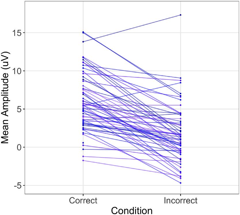
H.I. Volpert-Esmond et al. International Journal of Psychophysiology 162 (2021) 145–156
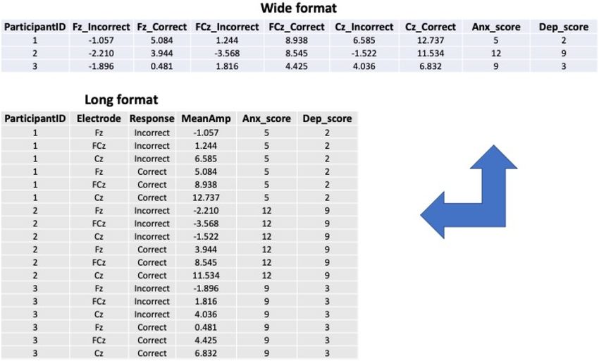
amplified with a Neuroscan Synamps amplifier (Compumedics, Inc.), variables in the model. A large body of literature describes the ERN as a
filtered on-line with a bandpass of 0.05–40 Hz at a sampling rate of 500 negative-going deflection that is larger following incorrect relative to
Hz. Electrode impedances were kept below 10 KΩ. Ocular artifacts (i.e., correct responses (Holroyd & Coles, 2002; Olvet & Hajcak, 2009; Yeung
blinks) were corrected from the EEG signal using a regression-based et al., 2004). To confirm this pattern in the example dataset, we first
procedure (Semlitsch et al., 1986). On each trial of the flanker task, need to set up our data in long format, which means each observation is
participants saw a horizontal string of five arrowheads facing to the left in a unique row with columns identifying each variable associated with
or right, in which the central arrowhead matched (congruent condition) each observation (e.g., participant number, response type, channel).
or did not match (incongruent condition) the direction of the four This is in contrast to wide format, which is typically used in rANOVA,
flanker arrowheads. Participants completed 200 trials total and were where each participant is in a unique row and columns represent both
allowed to rest every 50 trials. On each trial, participants first saw a different variables and repeated observations (see Fig. 2 for an illus
fixation cross (jittered: 1400 ms, 1500 ms, 1600 ms), followed by the tration). We can also include individual differences variables as unique
string of arrows (100 ms). Participants had 800 ms from the onset of the columns (e.g., anxiety and depression scores). Since each participant has
stimulus to identify the direction of the target (central) arrowhead with only one value for each individual difference variable, that value is
their right or left index fingers using a game controller. If they did not repeated for every row associated with a particular participant when the
respond within the 800 ms response deadline, a ‘TOO SLOW’ message data is in long format.
was presented on the screen before the next trial.
Following baseline correction (baseline window: − 300 to − 100 ms 2.1. Setting up the model
prior to the response), error trials and correct trials were averaged
separately to create two averaged waveforms per participant (see Fig. 1). To fit the model, we will use the lme4 (Bates et al., 2015) and
Trials where no response was made and trials containing deflections lmerTest (Kuznetsova et al., 2017) packages in R. All R code is down
±75 μV were not included. Only participants with more than 6 artifact- loadable at [https://github.com/hivolpertes/MLMbestpractices]. First,
free error trials were included in the analysis (Olvet & Hajcak, 2009), we need to determine the hypothesis we want to test, and thus the
resulting in a sample of 60 participants (19 male, 39 female, 2 trans/ outcome variable and the fixed effects or predictor variables to include
non-binary) for the analysis. We quantified the ERN/CRN as the mean in the model. In this example, we want to test differences in the mean
amplitude from 0 to 100 ms following incorrect/correct button presses, amplitude of the ERN/CRN following incorrect/correct responses. Thus,
respectively, at channels Fz, F1, F2, F3, F4, FCz, FC3, FC4, Cz, C1, C2, mean amplitude of the ERN/CRN is the outcome variable and response
C3, and C4. In addition to the flanker task, participants completed (e.g., incorrect, correct) is the predictor (or fixed effect).
several self-report measures, including symptoms of anxiety and Then, we must specify which random factors and structure to use,
depression using the GAD-7 (Spitzer et al., 2006) and PHQ-9 (Kroenke & which reflects the hierarchical nature of the data. This includes which
Spitzer, 2002), respectively. grouping variables (alternatively called random factors) to include and
As with any other analytic strategy, the first thing to do is determine which slopes and intercepts you allow to vary for each random factor.
the theoretical hypothesis to test, including the predictor and outcome ERP studies using averaged waveforms often have multiple observations
for each channel and for each participant and thus, the most common
random factors are participants and channels. Participants and channels
can either be specified as independent factors (i.e., cross-classified
model) or channels can be nested within participants (i.e., hierarchical
model). A hierarchical model assumes that lower-level units (in this
case, channels) belong to one and only one higher-level unit (in this case,
participants). This might be the case if you expect the placement of the
cap on each participant to vary, such that Fz measured for one partici
pant is substantially different from Fz measured for another participant.
In contrast, a cross-classified model assumes that lower-level units do
not belong to one and only one higher level unit.
Additional random factors can be selected depending on the data set
and theoretical hypothesis being tested, such as stimulus items. Impor
tantly, any random factor should contain enough units or clusters that
observations are clustered within, although the threshold of what is
enough is debated and depends on what estimated parameter you are
most interested in (Gelman and Hill, 2007; Huang, 2018; McNeish and
Stapleton, 2016a, 2016b; Snijders and Bosker, 1999). In general, the
fewer the units or number of clusters within a random factor, the poorer
the estimation of the variance associated with the random factor (Maas
and Hox, 2005). A common rule of thumb is the 30/30 rule (30 units or
clusters with 30 observations within each cluster). However, when
examining fixed effects, others recommend a minimum threshold of 10
(Snijders and Bosker, 1993), some suggest a minimal threshold of 5
when examining fixed effects but 10–100 when examining random ef
fects (McNeish and Stapleton, 2016a), and others suggest that having
fewer than 5 units within a random factor does no harm but also does not
differentiate the multilevel model from a classical regression model
when examining the fixed effects (e.g., Gelman and Hill, 2007). Since
most ERP studies using MLM are primarily interested in the fixed effects,
we recommend including measurements from at least 5 units or clusters
within a random factor (e.g., at least 5 channels in order to use channel
as a random factor). In the current example, we have repeated mea
Fig. 1. Averaged waveforms from example dataset (ERN-CRN). surements within channels (13 channels total) and participants (60
147
H.I. Volpert-Esmond et al.                                                                                    International Journal of Psychophysiology 162 (2021) 145–156

                                                     Fig. 2. Illustration of wide and long data formats.

participants total), so both are used as random factors. Since the same             to estimate random intercepts for each participant. If you think that the
channels are being used for all participants, and we expect channels                effect of a particular predictor on the outcome will differ across people
measured for one participant to be the same as for another participant,             in either size or direction, then you will want to estimate a random slope
we will use a cross-classified model for this example.                              for that particular predictor by participant. Similar justifications can be
    Now that we have our random factors, we can think about which                   made for including random intercepts and slopes for other random
variables correspond to each level of the model. Level 1 variables                  factors, such as channels. However, given that adjacent electrodes are
correspond to individual observations, such as response type, other                 theorized to measure similar brain activity, the effect of a predictor is
experimental manipulations, or aspects of the stimuli or trials that are            not often expected to differ across channels and random slopes are not
included as predictors. Level 2 variables correspond to one level above             often used in this case. Thus, one way to make decisions about random
that. In a cross-classified model where participants and channels are               effects specification is based on past empirical data or theory.
crossed random factors (and on the same “level,” so to speak), variables
corresponding to either participants or channels are Level 2 variables. In          2.1.2. Empirical approach
a hierarchical model where channels are nested within participants,                     Of course, your theory may be wrong (or limited). Within the last
variables corresponding to channels are Level 2 variables and variables             decade, researchers in psycholinguistics began calling for researchers to
corresponding to participants are Level 3 variables.                                follow a data-driven procedure where the maximal random effects are
    Once you have chosen your random factors and decided to use a                   specified for every model (“maximal model;” Barr et al., 2013). In a
hierarchical or cross-classified model, you must decide which slopes and            maximal model, all Level-1 predictors3 are specified as random slopes.
intercepts will vary by random factor. In general, allowing the effect of a         However, others have noted that using maximal models can result in
variable to vary by a random factor (i.e., including it as a random slope)          significant loss of power (Matuschek et al., 2017). Additionally, as noted
will not affect the estimate of the fixed effect for that variable, because         by Barr et al. (2013), the maximal model is frequently too complex to
the fixed effect is essentially the average of the random slopes. However,          properly converge. When the maximal model is too complex to
including a random slope will generally expand the standard error of the            converge, parameter estimates are incorrect and models must be
fixed estimate, thus increasing the associated p-value (Barr et al., 2013;          simplified. Thus, the maximal model may not always be appropriate and
Gelman and Hill, 2007). In other words, including a random slope                    parsimonious models may be preferable. To determine the most
(especially when there is a lot of group-related variance) controls the             appropriate parsimonious models, a number of strategies are used,
Type 1 error rate of the test of the fixed effect more tightly and provides         including comparing nested models using likelihood ratio tests (for a
a more conservative (and, some argue, more appropriate) test (Heisig                comparison of strategies for model selection, see Seedorff et al., 2019).
and Schaeffer, 2019). When choosing which effects to include as random
slopes, you can use either a theory-driven approach or an empirical or
data-driven approach.                                                                3
                                                                                        This applies only to Level-1 predictors, as Level-2 predictors cannot be
                                                                                    included as a random slopes within a Level-2 random factor, because they are
2.1.1. Theory-driven approach                                                       invariant within Level-2 units. In other words, if participants are being used as a
    A linear model is a formal representation of a hypothesis, which                random factor, Level-2 predictors (like depression or anxiety scores) will only
extends to how you believe units within a random factor differ from one             have one observation for each person, so the effect of these variables on the
another. If you think that people differ in terms of the outcome variable           outcome cannot be estimated separately for each person. In order to estimate a
(e.g., average amplitude of a given ERP component), then you will want              different random slope for each unit in a random factor, you need at least two
                                                                                    observations per unit.

                                                                              148
H.I. Volpert-Esmond et al. International Journal of Psychophysiology 162 (2021) 145–156
Regardless of whether you use a theory-driven or empirical approach to distribution to the Wald t values, Markov-chain Monte Carlo (MCMC)
specify random effects, we believe that best practices involve at mini sampling, parametric bootstrapping, and different approximations for
mum including random slopes for the main fixed effects of interest to denominator degrees of freedom. We recommend the Satterthwaite
properly control for Type 1 error, as intercept-only models are approximation for denominator degrees of freedom, partly because it
frequently too liberal and may result in spurious findings (Bell et al., more appropriately controls Type 1 error and is less dependent on
2019). Once you have accounted for the main fixed effects of interest, sample size than other methods, especially for REML-fitted models
you can make decisions whether to include more complex interactions as (Luke, 2017) and because of the ease of implementation—Satterthwaite
random slopes using a data-driven approach. approximation is the default for SAS and can be applied in R using the
Last, after having determined the fixed effects and random effects, lmerTest package (Kuznetsova et al., 2017) in conjunction with the lme4
you should choose the type of variance-covariance matrix to use, which package (Bates et al., 2015). All examples presented in this paper use the
specifies assumptions about how observations within and across units in Satterthwaite approximation when reporting p values.
a random factor (e.g., within and across participants) vary and covary. Critics of NHST suggest that whether the effect of a particular pre
Some variance-covariance matrices involve more stringent assumptions, dictor is different from zero is not always informative—instead, it may
such as a compound symmetry variance-covariance matrix, which more be more useful to understand the proportion of variance explained by
closely approximates a rANOVA. We suggest using an unstructured the fixed effects (and therefore make judgements of the meaningfulness
variance-covariance matrix, which removes the sphericity assumption of of the effect). In a single level regression or GLM, readers are familiar
rANOVA, as the assumption of sphericity is unrealistic when applied to with R2 as the variance explained by all of the fixed effects included in
psychophysiological data (e.g., Blair and Karniski, 1993; Jennings and the model. However, in multilevel models, the variance explained is a
Wood, 1976; Keselman and Rogan, 1980; Vasey and Thayer, 1987). By little more complex, since there are now multiple residual terms. Thus,
default, the lme4 package in R uses an unstructured variance-covariance several methods of calculating a pseudo-R2 have been proposed (e.g.,
matrix, although SAS by default uses a VC variance-covariance matrix Edwards et al., 2008; Johnson, 2014; Nakagawa et al., 2017; Nakagawa
(for more information on variance-covariance matrixes, see Haverkamp and Schielzeth, 2013; Snijders and Bosker, 1999). Importantly, there is a
and Beauducel, 2017; Page-Gould, 2017). distinction between the marginal R2, which is the proportion of the total
As mentioned before, in our example, we are testing the effect of variance explained by the fixed effects, and the conditional R2, which is
Response Type (RespType) on the mean amplitude of the ERN/CRN. The the proportion of the variance explained by both fixed and random ef
model includes two crossed random factors (Participant, Channel), fects. Either the marginal or conditional R2 can then be converted to
which we are estimating using an unstructured variance-covariance other effect sizes that may be more common in your particular research
matrix. Using a theory-driven approach to determine the random ef literature. For example, the model R2 can be used to compute Cohen’s f2
fects, we included 1) a random intercept by participant, 2) response type (Cohen, 1992) using:
as a random slope by participant, and 3) a random intercept by channel.
R2
The full model is described using Wilkinson notation as: f2 =
1 − R2
MeanAmp̃RespType + (RespType|Participant) + (1|Channel)
To estimate the variance explained by a particular predictor (i.e., to
Our interpretation of the fixed effects depends on how Response obtain an estimate of the local effect size), several methods exist. One
Type is coded, similarly to interpreting fixed effects from a single-level method is to estimate Cohen’s f2 for each local effect by estimating R2 for
regression model. When Response Type is dummy-coded (correct = 0, two nested models:
incorrect = 1), the estimate of the intercept is b = 5.926, 95% CIs [4.51,
R22 − R21
7.34] and the estimate of the effect of Response Type is b = − 4.294, 95% f2 =
1 − R22
CIs [− 5.20, − 3.39]. From these estimates, we can calculate the esti
mated marginal means for each group: the estimated marginal mean in where R22 represents the variance explained by a model with the effect of
the correct condition is 5.926 μV (the estimate of the intercept, since interest (the full model) and R21 represents the variance explained by a
correct is coded as 0) and the estimated marginal mean in the incorrect model without the effect of interest (the restricted model). Cohen’s f2 for
condition is 1.632 μV (the estimate of the intercept minus the estimate of a local effect can easily be directly calculated using this method in SAS
Response Type). When Response Type is effect-coded (correct = − 1, (Selya et al., 2012) and in R by fitting each model separately and esti
incorrect = 1), the estimate of the intercept is b = 3.779, 95% CIs [2.42, mating the pseudo-R2 as mentioned previously using the r.squar
5.13] and the estimate of the effect of Response Type is b = − 2.147, 95% edGLMM() function in the MuMIn packag (Bartoń, 2020) or the r2beta()
CIs [− 2.60, − 1.69], which means that across all trials, the estimated function in the r2glmm package (Jaeger, 2017).
marginal mean is 3.779 μV. Then, we can calculate the estimated mar An alternative method is to calculate a partial R2 statistic for each
ginal means for each condition by adding or subtracting the estimate of predictor, R2β (Edwards et al., 2008). One R2β statistic can be calculated
Response Type to the intercept, which gives us the equivalent marginal for each predictor using the ANOVA output of an MLM model to get the
means for correct and incorrect trials as the dummy-coded model. Using F-statistic, the numerator (effect) degrees of freedom, and the denomi
unstandardized estimates in this way gives us a sense of the magnitude nator (residual or error) degrees of freedom that correspond to each
of the difference between conditions in a meaningful unit (μV). When predictor.
examining latency as the outcome variable, estimates similarly can be ( )
interpreted in whichever meaningful unit the outcome variable was df numerator
F
measured on (such as milliseconds). df denominator
R2β = ( )
Researchers using the null hypothesis significance testing (NHST)
1 + dfdf numerator F
approach will additionally want to know if the effect of Response Type is denominator
statistically different from zero. Compared to single-level regression,
In the realm of ERPs, it remains unclear how large of an effect is
determination of degrees of freedom (and thus, the p-value associated
meaningful, as meaningful differences in amplitude may vary depending
with a test of a fixed effect) is much more complicated in MLM. A
on the ERP component of interest and the variance in the outcome is
number of possibilities exist for testing the significance of a fixed effect,
related to a number of factors, including the noisiness of the data and
including likelihood ratio tests of nested models, applying the z
how many trials are included in each averaged waveform. Thus,
149H.I. Volpert-Esmond et al. International Journal of Psychophysiology 162 (2021) 145–156
descriptions of effect size in future ERP studies are essential to trian
gulate what may be a meaningful effect size in the study of ERPs.
3. Visualizing data
In addition to statistical tests, visualizing data is an important
component of understanding statistical results. As most ERP studies are
interested in the effect of categorical predictors, a common approach
using rANOVA is to use bar or line graphs to depict mean amplitude
averaged across participants and channels in each condition. However,
depicting averages from the data does not account for the multilevel
structure of the data, nor does it depict how much variability in the
effect exists across people. When using multilevel modeling, we can plot
1) the fixed effects estimates to summarize patterns across the whole
sample, 2) the variance within each grouping variable (e.g., how par
ticipants vary from each other), or both. To plot mean differences across
experimental conditions and still account for the multilevel structure,
we can plot the model-estimated means from the fixed effects (alterna
tively called estimated marginal means). For both bar and line charts, Fig. 4. Spaghetti plot illustrating variance in effect of Condition across par
this should include the values of the outcome variable that are predicted ticipants (i.e., random slopes).
from your model for each condition (i.e., estimated means) and the
standard errors of these model-estimated means as error bars. Estimated
means can be calculated using a user-friendly, online tool available at
Of course, one can also plot both the estimated means for each
http://www.quantpsy.org/interact/ (Preacher et al., 2006) or the
condition and variance across individuals by overlaying the two plots.
emmeans package in R (Lenth, 2020) and then plotted as in Fig. 3.
We suggest plotting the “average” effect (i.e., the fixed effect) in a
However, one benefit of MLM is being able to estimate unique effects
slightly thicker width or different color to make it stand out (e.g., see
for each unit in a random factor (e.g., participant) by including random
Fig. 5).
slopes in the model. To visually represent the variance in a particular
effect, plot the best linear unbiased predictions (BLUPs) estimated for each
4. Extended applications of MLM
participant using a “spaghetti plot”. Spaghetti plots illustrate the vari
ance in the effect, which we can see in differences in the slopes of the
One of the major benefits of MLM that rANOVA cannot accommo
lines. If all lines are relatively parallel, there is little variance in the effect
date is including continuous variables in the model. One example of this
of Response Type across participants (which will be reflected in a small
is testing how individual difference variables moderate the effect of the
estimate of variance of the random slope of Response Type by partici
manipulated predictor. Past work has shown a link between trait anxiety
pant), whereas lots of intersecting lines that are not parallel suggest a
and the size of the ERN/CRN, such that those who are more anxious
large amount of variance in the random slope. We suggest plotting each
show a more pronounced negativity following errors (Hajcak et al.,
line with an opacity level below 100% to make each line easier to see
2003; Weinberg et al., 2010; Meyer, 2017). To test the effect of trait
and consider making each line its own color, if color visualizations are
anxiety on the size of the ERN/CRN using MLM, we can simply include
an option for your publishing outlet of choice (see Fig. 4 for an example).
trait anxiety as a predictor in the model (Response Type is effect coded;
As we can see in this example, most participants show the same pattern
Correct = − 1, Incorrect = 1):
as the fixed effect (more negative ERN amplitude in the incorrect con
dition compared to the correct condition), but some slopes are flatter
than others, and some participants even show an effect in the opposite
direction.
Fig. 5. Spaghetti plot with model estimated means overlaid.
Note. The thick black line represents the average relationship estimated by the
fixed effect and the thinner, multicolored lines represent the specific relation
Fig. 3. Model-estimated means plot illustrating fixed effect of response type. ships estimated for each person (the random slopes).
150H.I. Volpert-Esmond et al. International Journal of Psychophysiology 162 (2021) 145–156
MeanAmp̃RespType ∗ Anx + (RespType|Participant) + (1|Channel) with its own set of challenges (Kristjansson et al., 2007; Tremblay and
Newman, 2015). By examining the fixed effect of time, or interactions
As mentioned in an earlier footnote, we would not include anxiety as
between time and other fixed predictors, researchers can infer large-
a random slope by participant because there is only one observation per
scale change in the amplitude or latency of ERP components over the
participant (and is thus invariant). In this model, the effect of Response
course of an experiment, as well as different rates of change for different
Type remains significant, b = − 1.87, 95% CIs [− 2.61, − 1.12], t(58.0) =
experimental conditions. Additionally, the variable indexing time can be
− 4.92, p < .001, such that mean amplitude is more negative following
included as a random slope by participant so that researchers can
incorrect responses than correct responses. The effect of trait anxiety is
examine how the effect of time (including processes such as habituation
marginally significant, b = 0.19, 95% CIs [− 0.01, 0.39], t(58.0) = 1.91,
or learning) differs across participants. To get estimates of individual
p = .061. Most importantly, to examine whether trait anxiety moderates
differences in the rate of change in ERPs, researchers can extract the
reactivity to errors, we would look at the Response Type x Anxiety
BLUPs, which are participant-specific estimates of the effect of time.
interaction. In this sample, the interaction is not significant, b = − 0.05,
However, including time as a random slope often results in non-
95% CIs [− 0.15, 0.05], t(58.0) = − 0.93, p = .356. The interaction
convergence issues, which must be addressed before interpreting the
provides a similar test as correlating trait anxiety scores with a differ
BLUPs. Last, using MLM with single-trial ERPs opens the door to using
ence score of the ERN and CRN (e.g., ΔERN). Previous research has
ERP amplitude or latency as a predictor of other trial-level variables
shown differences in ΔERN between anxious and control groups
(such as reaction time or other downstream ERP components; Volpert-
(Ladouceur et al., 2006; Pasion and Barbosa, 2019; Weinberg et al.,
Esmond and Bartholow, 2020; Von Gunten et al., 2018).
2010, 2012, 2015) and significant relationships between symptoms of
Including continuous variables introduces increased complexity
generalized anxiety disorder and ΔERN (Bress et al., 2015; Klawohn
surrounding issues of centering variables that are unique to MLM. In
et al., 2020), such that more anxious participants show a more negative
typical single-level OLS regression, researchers often center and/or
ERN relative to the CRN, although other studies have not found
standardize continuous variables in order to interpret all other fixed
consistent significant correlations between self-reported anxiety and
effects as the effect observed at the mean of the centered variable. We
ΔERN (e.g., Meyer et al., 2012).
suggest taking a similar approach to all continuous Level 2 variables (e.
Another application that MLM allows for is the investigation of ERP
g., individual difference variables). However, in multilevel data,
responses to specific stimuli or events from individual trials, allowing
continuous Level 1 variables can either be centered across the entire
researchers to investigate how ERP signals meaningfully change over the
data set (grand-mean centering) or centered within each level of the
course of different trials or meaningfully differ in response to specific
grouping variables (group-mean centering). The type of centering one
instantiations of stimulus presentations. As mentioned previously, prior
chooses can significantly impact the interpretation of the fixed effects.
to data analysis researchers typically average all responses elicited by
There are a number of other resources discussing centering (e.g., Brauer
stimuli of the same type or experimental condition (i.e., signal aver
and Curtin, 2018; Enders and Tofighi, 2007; Kreft et al., 1995; Paccag
aging; Luck, 2014), which results in a data structure in which each
nella, 2006; Page-Gould, 2017) and contrast coding (Schad et al., 2020)
participant has a single observation per channel for each experimental
within multilevel data.
condition. This technique is effective for isolating physiological re
One particular case of centering that may be of interest may be dis
sponses to events of interest (i.e., increasing signal-to-noise ratio) but
aggregating between- and within-participant effects of a continuous
makes assumptions that might not be tenable, including that the signal is
predictor (e.g., Curran and Bauer, 2011). This is particularly relevant
constant across trials, and that any trial-to-trial variation is solely the
when using single-trial ERPs as a continuous predictor of some other
result of noise, and therefore meaningless. A number of factors,
outcome, such as a behavioral response within the same trial or an ERP
including habituation, fatigue, sensitization, or momentary lapses in
response on a subsequent trial. In the absence of disaggregation, the
attention can result in meaningful variation (i.e., not merely noise) in
relationship between single-trial ERPs and reaction time (for example)
ERPs across trials, thereby undermining the validity of signal averaging
conflates the between-person effect (i.e., Do people with particularly
in some situations.
large ERP responses also respond faster to stimuli in a particular task?)
A number of approaches to analyzing single trial ERPs have been
and the within-person effect (i.e., Does a larger ERP response on a
proposed (Blankertz et al., 2011; Coles et al., 1985; Debener et al., 2005;
particular trial, relative to a person’s average ERP response, facilitate a
Gaspar et al., 2011; Jung et al., 2001; Pernet et al., 2011b; Philiastides
faster reaction time?). Depending on the theoretical question, re
et al., 2006; Quiroga and Garcia, 2003; Ratcliff et al., 2009; Regtvoort
searchers may be more interested in one relationship than the other. To
et al., 2006; Rousselet et al., 2011; Sassenhagen et al., 2014). Multilevel
disaggregate within- and between-person effects, the researcher can
modeling provides an extremely useful additional tool for researchers
effectively separate the predictor variable of interest into two separate
interested in trial-level variation in ERPs. Note, however, that because
predictors. The first predictor—each participants’ mean—is entered as a
noise is not first being removed from the waveforms using the signal
Level-2 (person level) predictor and represents the between-person ef
averaging approach, it is important that the EEG data are as clean as
fect. The second predictor—the participant-centered variable—is
possible when a trial-level approach is used. Researchers should spend
entered as a Level-1 predictor and represents the within-person effect.
additional time and effort during the data collection process to ensure
the highest quality data possible to reduce noise in the data and increase
5. Reporting practices
the ability of multilevel models to detect fixed effects of interest from
individual trials.
Because of the complexity surrounding MLMs, researchers have a
To examine the linear effect of time on change in psychological
number of degrees of freedom with respect to how MLMs are estimated
processes, researchers can include time or trial number as an additional
and reported, including what covariance structure to use, which vari
fixed predictor in the model (e.g., Berry et al., 2019; Brush et al., 2018;
ables to include as fixed and random effects, how to test for interactions,
Volpert-Esmond et al., 2018). As an example, the model may be speci
how to center or effect-code variables, etc. Because of the flexibility of
fied as:
these models, it is imperative to provide enough information for an in
DṼIV + Trial + (IV|Participant) + (1|Channel) dependent party to replicate the analysis and evaluate its suitability for
the dataset at hand. Of course, providing code in an online repository
Note that the inclusion of Trial in this way can only capture long-
such as Open Science Framework or GitHub is preferable. But we
range trends such as habituation and fatigue. Quadratic and other
encourage researchers to include all essential information in the
non-linear effects can be included as additional predictors, although
manuscript as well. At minimum, the entire model, including variance-
little research has been done in this area and polynomial fitting comes
covariance structure and random effects should be described (Meteyard
151H.I. Volpert-Esmond et al. International Journal of Psychophysiology 162 (2021) 145–156
and Davies, 2020). To most effectively communicate the structure of
each model used, we suggest using Wilkinson notation, which specifies 8.314
ICCpar = = 0.77
the DV, IVs, and random effects. For example, 8.314 + 0.141 + 2.306
DṼIV1 + IV2 + (1 + IV1|Participant) + (1|Participant : Channel) 0.141
ICCelec = = 0.01
8.314 + 0.141 + 2.306
specifies that two predictors were included, but not their interaction;
that the intercept and the effect of the first predictor was allowed to vary In other words, variance between people accounts for 77% of the
by participant (i.e., IV1 was included as a random slope by participant); total variance, suggesting there is a lot of between-person variability in
and that the intercept was allowed to vary by channel nested within ERPs, whereas variance between channels accounts for 1% of the total
subject. Alternatively, the following model specifies participants and variance, suggesting is there not a lot of variability between channels,
channels as crossed random factors: which is expected given similarities in waveforms at adjacent channels.
In contrast, when using trial level data, the ICC associated with subject is
DṼIV1 + IV2 + (1 + IV1|Participant) + (1|Channel) 0.09, suggesting between-person variability only accounts for 9% of the
R users will recognize that Wilkinson notation is used in the lme4 total variance. Because of the amount of within-person variance from
package to specify models (and is also used in Matlab), thus providing trial to trial, between-person variance accounts for much less of the total
less of a barrier than formal mathematical notation. The statistical variance when using single-trial ERPs instead of signal-averaged ERPs.
software used to fit the models should additionally be reported, along
with any changes to the default specifications (e.g., which covariance 6. Estimating power
structure is specified). More extensive recommendations about report
ing practices regarding model selection, model output, etc., can be found Another barrier in transitioning to using MLM is the daunting pros
in Meteyard and Davies (2020). pect of having to do a power analysis. Evaluating the power of a hy
In addition to reporting the structure of the models using Wilkinson pothesis test, which is defined as the probability that the test will
notation, we suggest reporting the intraclass correlation coefficient correctly reject the null hypothesis when the null hypothesis is false, is
(ICC) for each random factor, which can be calculated from the vari important in assessing how likely a particular result is true and able to be
ances estimated in the random effects: replicated. Additionally, ERP studies are often underpowered to find
small effects (Clayson et al., 2019). Given that estimating an effect of
τ2 zero—or estimating effects completely at random—is more accurate at
ICC =
τ2 + σ 2 determining the true population mean than using sample means derived
from poorly powered studies (Davis-Stober et al., 2018), and that EEG
where τ2 is the between-cluster variance (the variance associated with
studies are time-intensive and costly to run, an a priori power analysis
the random factor) and σ2 is the residual variance (Lorah, 2018). This
can inform a researcher whether they have the resources to conduct a
gives you the proportion of total variation in the data that is accounted
study that is well-powered enough to be informative. Additionally, ac
for by a particular random factor where higher ICCs represent more
cording to recent guidelines for best practices in reporting of ERP studies
variance between units within that random factor (Gelman and Hill,
(Keil et al., 2014), researchers should always report the achieved power
2007). Since the complexity of the model affects the calculation of ICC,
of a particular design. Many tools are available to estimate power for
you should use variance estimates from an intercept-only model (i.e., a
typical single-level designs (e.g., Faul et al., 2009; Murphy et al., 2014),
model with no fixed predictors):
although discussion is still ongoing about the most appropriate ways to
DṼ1 + (1|Participant) + (1|Channel) conduct and use a power analysis (Anderson et al., 2017; Cribbie et al.,
2019; Albers & Lakens, 2018; Lakens & Evers, 2014).
When including more than one random factor (e.g., including par
In multilevel designs, how power relates to sample size is more
ticipants and channels in a cross-classified model), one would include
complicated, as both the number of groups (e.g., the number of in
the variance of all groups in the denominator. As an example, let’s look
dividuals who participate during the study) and the number of obser
at sources of variance in the mean amplitude of the P2 ERP component
vations per group (e.g., the number of trials or observations per
elicited by Black and White male faces during a race categorization
individual) can vary. In multilevel models, power is affected by group
task.4 To calculate the ICC associated with subject, we would look at the
sample size, observation sample size within each group, the ICC asso
output for the random effects from the following intercept-only model,5
ciated with group, whether you are testing a Level 1 (observation-level)
first using the signal averaged data:
or Level 2 (participant-level) effect, and numerous other parameters of
Model : P2amp̃1 + (1|Participant) + (1|Channel) the model (Arend and Schäfer, 2019). As a general rule of thumb,
increasing the number of Level 2 units (e.g., the number of people
Random effects output:
participating in the study) has a larger effect on power to detect fixed
Random factors Name Variance Std. dev.
effects than increasing the number of Level 1 units (e.g., the number of
Participant (Intercept) 8.314 2.883 experimental conditions or trials within each participant; Maas and Hox,
Channel (Intercept) 0.141 0.376 2005; Snijders, 2005). For a more specific approximation of the sample
Residual 2.306 1.5184
size (at both Level 1 and Level 2) needed to achieve the desired level of
power for a particular test, most researchers use a simulation approach
to power using Monte Carlo simulations. This approach repeatedly
4
Data were previously published in Volpert-Esmond et al. (2017). Although simulates data from the hypothetical distribution that we expect our
the original study manipulated where participants fixated on the face, data used
sampled data to come from and then fits the same multilevel model to
here include only trials presented so that participants fixated in a typical
each data set. Power is estimated by how often the true effect is detected.
location (i.e., between the eyes). The sample includes 65 participants and the
average number of trials included per participant was 107.7 (min = 54, max =
To set up a power simulation, you need to make assumptions about
127). Data from 7 channels were used (C3, C4, CP3, CP4, CPz, Cz, Pz). the true treatment effect and also specify all the other parameters that
5
This is an example of a cross-classified model, where subject and channel characterize the study, including the size of the fixed effect of interest,
are included as separate grouping variables, rather than channel being nested ICCs of any random grouping variables, variances of random intercepts
within subjects in a typical hierarchical model. Calculating ICCs for groups and slopes, correlations between random intercepts and slope, etc.
nested within each other is similar (i.e., estimates of variance for all groups plus Because of the large number of parameters needed to simulate an
the residual variance is used in the denominator).
152H.I. Volpert-Esmond et al. International Journal of Psychophysiology 162 (2021) 145–156
appropriate data set, it is often easier to conduct a power simulation on a
set of pilot data, although parameters can be assumed and simulated
without pilot data (Gelman and Hill, 2007). The simr package in R
(Green and MacLeod, 2016) has emerged as a popular tool for power
simulations using multilevel models. The package allows users to input a
sample data set (either a pilot or simulated data set) and calculate
observed power for a desired effect, as well as produce power curves in
which power is plotted as a function of a particular aspect of the design,
such as number of participants, number of observations within each
participant, or effect size. To provide an example of a power curve
generated using simr, we use previously published data6 looking at how
the race of a face influences mean P2 amplitude:
Model : P2amp̃Race + (Race|Participant) + (1|Channel)
When using signal averaged data, the effect of race is significant, b =
− 0.59, t(64.0) = − 4.82, p < .001, such that Black male faces elicit larger
P2s than White male faces. A post-hoc power simulation indicates that Fig. 7. Power to detect the fixed effect of race on P2 amplitude as a function of
the observed power for this effect with the given sample size (65 par effect size.
ticipants, 7 channels for each participant, and 2 observations for each Note. 14 observations are included for each participant (7 channels with 2
channel) is 99.6%, suggesting this design is very well-powered to detect observations at each channel). The sample size is set at 65 participants.
this effect. Fig. 6 shows a power curve demonstrating the decrease in
power as the sample size decreases.
Thus, we achieve 80% power to detect an effect of this size with
about 25 participants. However, using pilot data to estimate the true with significant limitations. First, effectively using MLM involves gain
effect size may result in an underpowered follow-up study (Albers & ing the expertise to organize data in the appropriate format, learning
Lakens, 2018; Anderson et al., 2017). Thus, we suggest either adjusting how to implement models in statistical software, making appropriate
the anticipating effect size to be smaller than that achieved in a pilot decisions for model specification, correctly interpreting the output, etc.
study when planning a follow up study or producing a sensitivity power Additionally, due to the continued evolution and development of
curve to identify what sample size would be needed to detect the knowledge about MLMs, there currently is a perceived lack of consensus
smallest meaningful effect size. Fig. 7 demonstrates the decrease in and established, standardized procedures (Meteyard and Davies, 2020).
power as the effect size decreases, indicating that with a sample of this Many resources are becoming available for researchers interested in
size, we would be able to detect an effect as small as b = − 0.35 with 80% learning this statistical approach, including workshops at prominent
power. conferences (i.e., Society for Psychophysiological Research), stand-
alone workshops hosted by societies, private organizations, and uni
7. Limitations versities (e.g., APA Advanced Training Institutes, Statistical Horizons,
University of Michigan, University of North Carolina, University of
MLM is not a panacea. As with any analytic approach, MLM comes Connecticut, Arizona State University), and numerous tutorials and ar
ticles on applying MLM to both behavioral data (Arnau et al., 2010;
Baayen et al., 2008; Brauer and Curtin, 2018; Gueorguieva and Krystal,
2004; Jaeger, 2008; Judd et al., 2012; Maas and Snijders, 2003; Quené
and van den Bergh, 2004, 2008) and psychophysiological data (Bagiella
et al., 2000; Kristjansson et al., 2007; Page-Gould, 2017; Tibon and Levy,
2015; Tremblay and Newman, 2015; Volpert-Esmond et al., 2018;
Vossen et al., 2011). However, little is known about the effectiveness of
this training and how it is implemented in practice (King et al., 2019).
Moreover, the mere fact that these opportunities exist does not ensure
that researchers will or can take advantage of them, and therefore this
situation is far from ideal in terms of ensuring adequate quantitative
methods training in the field—likely contributing to a significant gap in
psychologists’ quantitative training. Thus, learning how to appropri
ately apply MLM to ERP data may be a significant barrier.
In addition to the time cost of learning the approach, MLM is often
quite computing-power intensive and models can take much longer than
a typical rANOVA to run. In the case of the P2 example given previously,
the first author ran these models on a MacBook Air with a 1.6 GHz Dual-
Fig. 6. Power to detect the fixed effect of race on P2 amplitude as a function of
Core Intel Core i5 processer with 8 GB of RAM. To test the effect of face
sample size.
race on P2 amplitude using signal-averaged data, it took only a few
Note. 14 observations are included per each participant (7 channels with 2
observations at each channel). The effect of race is set at b = − 0.59 (the seconds to fit the model. To run the same model using trial-level data, it
observed effect size in the data). took less than 10 s to fit the model. However, as the data set becomes
larger and the model becomes more complex, the time required to fit a
MLM increases dramatically. For example, this more complex model
testing the effect of target race, target gender, fixation, task, and
participant race on trial-level P2 data recorded in two face processing
6
Same data as used in ICC example.
153You can also read