How Essential Is Essential Air Service? The Value of Airport Access for Remote Communities

How Essential Is Essential Air Service?
 The Value of Airport Access for Remote Communities
 Austin J. Drukker
 University of Arizona
 January 2023
 Essential Air Service is a federal government program that provides subsides to airlines that
 provide commercial service between certain remote communities and larger hubs, which
 proponents argue are justified because driving to larger airports would be prohibitively
 expensive for residents of these communities. I estimate the value of Essential Air Service to
 local communities using a revealed-preferences approach by formulating and estimating a
 discrete-choice model of domestic air travel purchases that incorporates passengers’
 geographical proximity to alternative airports. I estimate the model using proprietary data
 containing millions of domestic airline passengers’ residential ZIP codes coupled with their
 choice of airline product. Simple data tabulations reveal that most travelers living in regions
 receiving subsidized service have several alternative airports to choose from and generally
 prefer to drive to larger airports. A counterfactual policy simulation using the estimated model
 finds that, in aggregate, community members value subsidized commercial air service from
 their local airport at $16 million per year, compared to an annual cost of over $290 million.
 Keywords: airport, airline, subsidy, public finance, substitution, discrete choice
 JEL Codes: H54, L93, R53

I. INTRODUCTION
 For the last half century, the US domestic aviation industry has operated in a largely unregulated market
environment. The Airline Deregulation Act of 1978 removed federal government control over fares, routes,
flight frequency, and the entry of new airlines, leading to improvements in service, decreases in fares, and
increases in the number of flights, passengers, and miles flown. Today, passenger aviation is a major
component of the modern global economy, contributing about 5 percent to US gross domestic product
annually (IATA, 2019; FAA, 2020). According to the International Civil Aviation Organization, 4.5 billion
passengers globally flew on scheduled air service in 2019, and the Federal Aviation Administration (FAA)
provides air traffic control services for more than 2.9 million airline passengers per day (FAA, 2022).
According to the Consumer Expenditure Survey, about 13 percent of US households purchased at least one
airline ticket in 2019 and spent an average of $3,873 on airfare.
 Although the Airline Deregulation Act was largely viewed as a success, there was fear among some at
the time of its passage that small communities would be left behind in its wake as airlines shifted their
operations to serve large, profitable markets. To assuage this fear, Congress established Essential Air
Service (EAS) in 1978, which required carriers to continue providing scheduled air service at pre-

 1

deregulation levels—typically two round trips per day—to eligible communities using subsidies if
necessary. Although EAS was originally set to expire after 10 years, under the assumption that air traffic
would eventually become self-sustaining, Congress reauthorized EAS for another 10 years in 1988 and
made it permanent in 1996. As of June 2022, costs for the program have ballooned to over $340 million
per year despite fewer communities being eligible today compared to in 1978. Given that EAS still exists
nearly a half century after Congress originally intending it to expire, it is reasonable to ask whether EAS
still achieves its stated purpose of efficiently and effectively connecting remote communities to commercial
air travel opportunities.1
 Understanding the value of EAS to the communities it serves requires understanding the trade-offs
faced by travelers. A key trade-off that community members face is whether to fly from their local airport,
which may be more convenient but offer fewer choices, or to drive to a larger airport, which may be far
away but offer more choices. To study this trade-off, I analyze proprietary choice data derived from credit
card transactions that link travelers’ airline product choices with their home ZIP code. The data, which have
not been used in any previous economic studies, allow me to easily compute travelers’ driving time to
alternative airports.2 Hence, driving time is an observable product characteristic whose marginal value to
consumers can be estimated using standard econometric techniques.
 The proprietary choice data reveal several important insights about airline markets previously not
known to researchers and policymakers. First, since I am able to directly observe which airports are chosen
by residents of a particular geographical area, it is relatively straightforward to determine which airports
effectively serve the same region.3 While the presence of multiple airports in a region does not in itself
imply that the airports provide substitutable services, the growth of air travel demand since the early 1990s
has attracted entry by airlines at different airports within the same region, suggesting a potentially important
role for spatial interactions in the airline industry that have been largely overlooked by previous research.4

1
 The Airline Deregulation Act (92 Stat. 1733) requires the Department of Transportation to “consider the desirability
of developing an integrated linear system of air transportation whenever such a system most adequately meets the air
transportation needs of the communities involved.”
2
 To my knowledge, only two academic papers (Yirgu and Kim, 2021; Yirgu, Kim, and Ryerson, 2021) have used
these data, and both papers use only a small geographical subset, in contrast to my data sample which covers the entire
United States from 2013 to 2019.
3
 See Fournier, Hartmann, and Zuehlke (2007). Studies that have considered regions with multiple airports vary widely
in which airports to include. Berry and Jia (2010, p. 11) consider six regions to have airports that are “geographically
close.” de Neufville (1995) lists nine regions served by more than one airport. Brueckner, Lee, and Singer (2014)
attempt to empirically estimate which airports serve the same metropolitan region based on competition spillovers and
specify 13 regions as having multiple competing airports. Drukker and Winston (forthcoming) consider 22 regions to
have multiple competing airports.
4
 Studies that consider aspects of spatial competition in non-airline markets include Manuszak and Moul (2009) and
Dorsey, Langer, and McRae (2022) (gasoline); Smith (2004) and Katz (2007) (supermarkets); Davis (2006) (movie
theaters); Ho and Ishii (2011) and Hatfield and Wallen (2022) (banking); and Murry (2017) and Murry and Zhou
(2020) (car dealerships). Studies that consider aspects of spatial competition in airline markets include Fournier,

 2

Relatedly, since I am able to observe the home ZIP code of an airport’s users, it is relatively
straightforward to determine the geographical boundary of an airport’s catchment area (the area from which
an airport draws its customers). Administrative and survey data from a variety of sources suggest that most
airports draw customers from a large geographical area, but most previous studies of the airline industry
have assumed airports have relatively small catchment areas, typically the geographical boundaries of a
city.5 Proper market definition is of first-order concern for almost any industry analysis because it directly
influences the scope of available substitutes for consumers and the degree of competition faced by suppliers.
Excluding certain viable airports from travelers’ choice sets may rule out important substitution patterns,
and estimates derived from narrowly defined choice sets will tend to overstate airlines’ market power by
understating travelers’ ability to substitute to alternative products, which in turn could have significant
implications for merger evaluations and antitrust enforcement.6
 The ability to view travelers’ choice sets is particularly useful for evaluating the costs and benefits of
EAS, since implicit in much of the debate surrounding the program is the assumption that members of
communities receiving EAS-subsidized service would have no other viable alternatives for accessing
commercial air travel apart from subsidized service from their local airport. My choice data allow me to
see which airports residents of an arbitrary geographical area actually use, allowing me to directly check
this assumption.7 Simple tabulations of the proprietary choice data reveal a key insight about the nature of
EAS community members’ choice sets, namely, that despite their ostensible isolation from the rest of the
national air transportation system, members of most EAS communities rarely choose to fly on EAS-
subsidized flights from their local airport and instead generally prefer to drive to airports of various sizes
offering more products with better characteristics. From an econometric perspective, failing to consider
these viable alternatives in travelers’ choices sets will make EAS appear more valuable than it actually is
because travelers will appear less price sensitive due to having fewer substitutes. From a policy perspective,

Hartmann, and Zuehlke (2007), Hess and Polak (2005, 2006), Ishii, Jun, and Van Dender (2007, 2009), Mahoney and
Wilson (2014), Brueckner, Lee, and Singer (2014), McWeeny (2019), and Drukker and Winston (forthcoming).
5
 Airlines For America’s 2019 annual survey found that 37 percent of passengers reported flying from an airport that
was not the closest to their home or office at some point in the previous year. McWeeny (2019) found that a significant
share of travelers surveyed at San Francisco International Airport drove from as far away as Sacramento (a 2-hour
drive) and that 57 percent of passengers surveyed at San Francisco International Airport bypassed an airport that was
closer to their home. Ishii, Jun, and Van Dender (2007) found that travelers located closest to San Francisco
International Airport most often departed from there, but passengers closest to San Jose International Airport or
Oakland International Airport often chose to fly from a different airport. Yirgu, Kim, and Ryerson (2021) report
significant airport leakage for small and medium-sized airports in the Midwest United States.
6
 The US Department of Justice uses a narrow city-pair market definition in cases involving airline mergers. See, for
example, their complaint against the proposed merger between American Airlines and US Airways (78 Fed. Reg.
71377) and their complaint against the Northeast Agreement between American Airlines and JetBlue Airways
(https://fingfx.thomsonreuters.com/gfx/legaldocs/zjpqkrdlmpx/plaintiffs-brief-american-airlines-2022.pdf).
7
 Bao, Wood, and Mundy (2015) and Lowell et al. (2011) compute the cost of subsidizing flights to the cost of
subsidizing bus service to the same location. They do not consider the costs of subsidizing bus service to alternative
airports.

 3

the revelation that EAS community members frequently choose to drive to alternative airports undermines
EAS’s raison d’être to provide an essential service to communities that would otherwise have no other
options to connect to the national air transportation system.8
 An added benefit of the proprietary choice data is that I can see the home location of any airport’s users,
which allows me to determine the extent to which an EAS-subsidized airport serves residents of the
community. Knowledge of the home location of EAS-subsidized airport users is policy relevant because
the purpose of EAS is to connect residents of the community to commercial air travel. Without the ability
to link purchases to the home location of purchasers, it would not be possible to determine who are the
primary users of EAS-subsidized service. Tabulations of the data reveal that the majority of EAS-subsidized
airport users are not residents of the communities in which the airport is located. This finding has important
fiscal policy implications because all users of EAS airports benefit from subsidized ticket prices, regardless
of residency status, implying a majority of EAS funds go toward subsidizing nonresidents of EAS
communities. The problem is further compounded by the fact that nonresidents who use EAS-subsidized
airports tend to have higher incomes than residents, which raises serious distributional concerns about the
program.
 To formally estimate the value that EAS community members derive from the program, I formulate
and estimate a discrete-choice model of air travel demand. I formulate my demand model using a nested
logit utility specification that closely resembles the canonical models of Berry, Carnall, and Spiller (1996,
2006) and Berry and Jia (2010). A key component of my model is the inclusion of driving time as a product
characteristic, which allows me to directly estimate the implicit monetary costs of driving to alternative
airports. I estimate my model using the generalized method of moments with a combination of macro and
micro data, as described by Berry, Levinsohn, and Pakes (2004) and Petrin (2002). Macro moments are
constructed using aggregate data containing information about airline products, their characteristics, and
the number of travelers who choose each product, and micro moments are constructed using the proprietary
choice data. Intuitively, the micro moments capture spatial variation between driving time and travelers’
choices (and non-choices), which is used to identify travelers’ preferences for driving.9
 A useful feature of the discrete-choice modeling framework is that it allows me to analyze
counterfactual policy experiments by estimating consumer surplus under two alternative scenarios. In
particular, I consider a counterfactual policy experiment in which all EAS subsidies are eliminated, which
would cause commercial service to cease at most airports currently served by EAS-subsidized airlines. The

8
 Grubesic and Matisziw (2011) thoroughly studied EAS community members’ access to a variety of alternative
airports, but their data do not allow them to study the extent of their use.
9
 McWeeny (2019) uses a similar revealed-preferences approach, which, unlike the stated-preferences approach used
by Landau et al. (2016), Daly, Tsang, and Rohr (2014), Adler, Falzarano, and Spitz (2005), Hess and Polak (2006),
and Hess, Adler, and Polak (2007), does not rely on self-reported or speculative valuations of trip components.

 4

difference between consumer surplus computed before and after the elimination of commercial service at
EAS airports reveals community members’ implicit value of the EAS program, and a simple comparison
between the costs and benefits of the program can be used to determine whether EAS subsidies are justified.
 I conduct my counterfactual policy experiment using data from 2019 for 107 EAS communities in the
continental United States. The analysis reveals that the members of these 107 communities collectively
value subsidized service from their local airport at $16 million annually, a paltry amount compared to EAS’s
cost in 2019 of over $290 million. Furthermore, this estimate likely overstates the effects of eliminating
EAS subsidies, since commercial service might not cease at all formerly eligible communities.
Disaggregating the results by airport reveals that desirable routes tend to be flown by legacy airlines
operating in a seemingly competitive environment, which is suggestive of rent-seeking behavior to the
extent EAS subsidies act as entry barriers for competitors.
 The remainder of this paper is organized as follows. In Section II, I provide a brief history and overview
of Essential Air Service. In Section III, I describe my data and present several novel insights based on
descriptive statistics. In Section IV, I formulate an empirical model of demand, and in Section V, I describe
the estimation strategy and sources of identification. In Section VI, I present the estimation results and
perform post-estimation checks. In Section VII, I present the results of my counterfactual policy analysis
to compute the consumer surplus that communities derive from EAS and consider distributional
implications. Section VIII concludes with a summary of the findings, policy recommendations, and
suggestions for future research.

II. ESSENTIAL AIR SERVICE

 The EAS program provides subsidies to airlines to provide regular service to eligible communities.10,11
To be eligible for EAS, a community must be located more than 70 miles from the nearest medium or large
hub airport, require a per-passenger subsidy rate of $200 or less ($1,000 or less if the community is farther
than 210 miles from a hub), and have 10 or more enplanements per day.12 EAS typically subsidizes one
airline to provide two to four round trips per day, six days per week, from an EAS community to a larger
hub. Although EAS eligibility is based on a community’s distance to the nearest medium or large hub,

10
 A handful of communities participate in the Alternate EAS program, which allows communities to forgo traditional
EAS for a prescribed amount of time in exchange for a flexible grant. In 2019, all communities participating in the
Alternate EAS used their funds to subsidize charter air service.
11
 EAS contracts do not give an airline the exclusive right to serve a community, and airlines may decide to serve a
community under an EAS contract without the use of subsidies.
12
 See Appendix C for a summary of the legal statutes and DOT practice regarding eligibility determination. Tang
(2018) provides an excellent primer on EAS, its history, and eligibility requirements.

 5

airlines that receive EAS contracts are not required to fly passengers to the nearest hub nor to a medium or
large hub.13
 Airlines compete for EAS contracts through a bidding process, and the DOT typically receives 1–3
proposals per airport every 1–3 years, when EAS contracts typically expire. By law, the DOT must take
into account the views of the community when deciding which proposal to accept, as well as the carrier’s
service reliability and any arrangements it has with larger carriers at the hub. Notably, subsidy cost is not
among the factors the DOT is required by law to consider when evaluating bids, and if more than one carrier
proposes to offer service then local officials are under no obligation to favor the proposal that entails the
lowest cost to the federal government.
 EAS has long been a target of critics who have derided the program as wasteful spending and an
inefficient means of connecting rural communities to commercial air travel, arguing that the statutes
governing EAS do not encourage cost efficiency and that the market, not government subsidies, should
decide which airports survive. But community stakeholders argue that EAS provides an essential service to
communities that would otherwise lose access to commercial air travel, arguing that EAS community
members value their local airport and without government subsidies the airport would cease to be
commercially viable. Several papers have argued that ending EAS subsidies would not necessarily reduce
service at eligible communities.14 But the question of whether and the extent to which EAS community
members value their local airport has not been studied and is one that I take up in the present paper.
 Figure 1 shows the locations of 107 airports receiving EAS-subsidized service as of September 2021.15
Following the Eno Center for Transportation’s (2018) convention, red dots represent communities that are
between 70 and 100 miles from a medium or large hub, orange dots represent communities that are between
100 and 150 miles from a medium or large hub, light blue dots represent communities that are between 150
and 210 miles from a medium or large hub, and dark blue dots represent communities that are more than
210 miles from a medium or large hub (DOT, 2021c). The green dots correspond to medium or large hubs
that are nearest to EAS communities or which are used by airlines serving EAS communities even if not
geographically closest (DOT, 2019a, 2022b).

13
 For example, Cape Air currently serves several EAS communities in Montana through their small hub at Billings
Logan International Airport. See Appendix C for the FAA’s definition of hub size.
14
 Cunningham and Eckard (1987) suggest that EAS subsidies may have actually reduced flight frequency because
EAS contracts serve as entry barriers that discourage competition. Morrison and Winston (1986) note that service to
small communities actually increased following deregulation—suggesting EAS subsidies mask profit opportunities.
Bao, Wood, and Mundy (2015) note 10 of the 34 EAS communities that have had their EAS subsides terminated since
1993 have experienced a substantial increase in their outbound passenger levels. Furthermore, subsidized airlines
currently provide commercial service alongside unsubsidized airlines at several EAS airports, most notably Allegiant
Air, which serves five currently eligible communities and one formerly eligible community.
15
 Appendix Table H3 lists the status of the 51 communities that have lost their EAS eligibility since 1989.

 6

Figure 1. The Locations of EAS Airports and Their Nearest Hubs

 Source: Federal Aviation Administration.
 Notes: Green dots are medium or large hubs that are geographically closest to EAS communities or are
used by EAS-subsidized carriers. Red, orange, light blue, and dark blue dots are EAS airports located less
than 70 miles, 70–100 miles, 100–210 miles, and more than 210 miles, respectively, from the nearest
medium or large hub.

 Although it would appear from Figure 1 that many EAS communities face considerable barriers to
access commercial air travel without the assistance of EAS, the color-coding belies the full picture by
restricting the notion of viability to medium hubs or larger. Figure 2 presents a fuller picture, augmenting
Figure 1 by including a host of viable airports that are classified as smaller than medium hubs. For example,
Figure 1 suggests Butte in southwest Montana is relatively isolated, located 6 hours to Salt Lake City to the
south and 10 hours to Portland or 9 hours to Seattle to the west. But Figure 2 reveals that there are four
additional airports within a 3-hour drive from Butte: Great Falls International Airport, Missoula Montana
Airport, Helena Regional Airport, and Bozeman Yellowstone International Airport, a small hub served by
8 major airlines flying to more than 20 destinations. The pink dots correspond to small hubs that are or have

 7

been used by airlines to serve certain EAS communities, but which are too small to factor into the distance
calculation for maximum allowable per-passenger subsidies.16

 Figure 2. The Locations of EAS Airports and Viable Nearby Airports

 Sources: Federal Aviation Administration; Airlines Reporting Corporation.
 Notes: See the notes to Figure 1. Pink dots are small hubs that are or have been used by EAS-subsidized
carriers. Purple dots are airports used by a nontrivial share of EAS community members.

16
 For example, Yellowstone Regional Airport in Cody, Wyoming, is only about 100 miles from Billings Logan
International Airport, but since Billings is considered a small hub it does not factor into the distance calculation; Salt
Lake City International Airport is the nearest large hub (about 450 miles away), so a carrier serving Yellowstone
Regional Airport would be exempt from the $200 per-passenger subsidy limit (DOT, 2019a).

 8

III. DATA AND DESCRIPTIVE STATISTICS

 Before describing the model and estimation strategy, I describe the data used to estimate the model and
present several figures showing the key features of the data. The data come from six primary sources. Table
1 (presented at the end of this section) provides summary statistics for several key variables.

A. Market Locator

 The primary data set used for the analysis comes from the Airlines Reporting Corporation’s (ARC’s)
Market Locator tool. Owned by the airline industry, ARC acts as a clearing system for all travel agencies,
including online travel agencies such as Booking Holdings, Expedia Group, and their subsidiaries, which
process about 35 percent of all domestic tickets sold in the United States. According to ARC, the clientele
is representative of the universe of domestic leisure and unmanaged business travelers.17 About 20 percent
of all tickets that come through the ARC clearing system are sent to a credit card processing company that
matches customers’ chosen product to their credit card billing ZIP code.18 The data are associated with the
point of sale of the airline ticket purchaser, which is likely to be the passenger in most cases.19 Thus, the
data are a roughly 7 percent representative sample of US domestic leisure passengers.
 The Market Locator data contain monthly passenger counts by ZIP code for 2013–19. Tabulations of
the Market Locator data reveal which airports travelers drive to without a priori selecting which airports to
include in a traveler’s choice set. For example, Figure 3 shows the 8 airports most commonly chosen by
residents of Decatur, Illinois and their respective market shares. In 2019, Cape Air received $3.065 million
to offer 24 nonstop round trips per week to O’Hare International Airport (ORD) and 12 nonstop round trips
per week to St. Louis Lambert International Airport (STL) from Decatur Airport (DEC), with fares to
Chicago starting at $59 one way and fares to St. Louis starting at $29 one way (DOT, 2017, 2019a; Cape
Air, 2018). According to the DOT (2019a), Decatur Airport had 17,066 passengers (both directions) in
2019, corresponding to a $180 per-passenger subsidy. Despite Cape Air offering unusually low prices,
tabulations of the Market Locator data reveal that only 7 percent of travelers flew from Decatur to either
Chicago or St. Louis, while 21 percent of travelers drove 2 hours and 15 minutes to St. Louis, 27 percent
of travelers drove 3 hours to Chicago, and 27 percent of travelers drove 1 hour to Central Illinois Regional

17
 As noted by Yirgu, Kim, and Ryerson (2021), business travelers are more inclined to purchase tickets directly from
airlines rather than through third-party agents, meaning they are less likely to show up in the Market Locator data.
18
 The ability to link tickets with billing ZIP codes is only limited by the credit card processing company used for the
transaction; otherwise, there are no selection criteria for determining which tickets can be linked with billing ZIP
codes. The credit card processing companies generally do not process American Express cards, so there is a slight bias
against business travelers to the extent business travelers are more likely to pay with American Express cards.
19
 Although the traveler’s point of origin is typically within proximity to the purchaser’s point of sale, this would not
be the case if, for example, the purchaser and passenger were in different locations or, more frequently, if the traveler
purchased one-way tickets individually.

 9

Airport (BMI), a non-hub primary commercial service airport served by four major airlines. The remaining
travelers drove to Springfield’s Abraham Lincoln Capital Airport (SPI), Urbana–Champaign’s Willard
Airport (CMI), Indianapolis International Airport (IND), or Peoria International Airport (PIA).

 Figure 3. Market Shares for Airports Chosen by Residents of Decatur

 Source: Airlines Reporting Corporation.
 Notes: See the notes to Figure 2. DEC is an EAS-subsidized airport in Decatur, Illinois. Market shares
conditional on flying are shown as percentages after the airport codes. The dotted lines indicate travelers
drove from Decatur to the indicated airport to take a departing flight. The dashed line indicates travelers
flew from DEC to the indicated airport en route to a final destination.

 The Market Locator data are also useful for determining who the primary users of an EAS-subsidized
airport are, namely, residents of the community or nonresident visitors. Knowing the home location of an
EAS airport’s users is policy relevant because the purpose of EAS is to connect EAS community members
to commercial air travel. To determine the residency status of EAS airport users, I draw geographical
boundaries around the communities as shown in Appendix B—typically the Metropolitan or Micropolitan
Statistical Area(s) encompassing the airport. Residents are then defined as passengers whose ZIP code is
within the geographical region, and nonresidents are those whose ZIP code is outside the region. Overall, I
find that nonresidents make up 57 percent of customers on EAS-subsidized flights. As shown in Appendix

 10

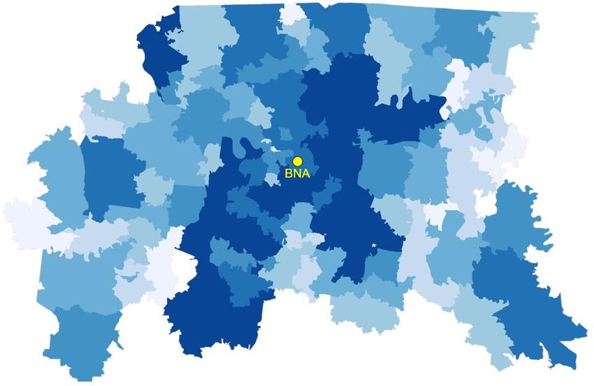
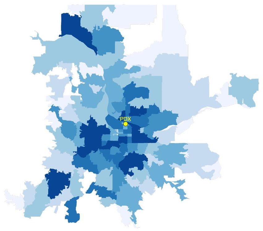
Figure H1 and Appendix Table H2, several EAS communities are located very close to national parks, and
airports in these communities likely serve as entry points for visitors; since all customers on EAS-
subsidized flights, regardless of where they live, benefit from lower ticket prices, it is plausible that EAS
serves to subsidizes tourism for these areas, which is not its statutory purpose. Yellowstone Airport, for
example, is used almost exclusively by tourists likely visiting Yellowstone National Park, while residents
of West Yellowstone overwhelmingly prefer to drive 1 hour and 30 minutes north to Bozeman Yellowstone
International Airport.20
 As will be explained in Section V.A, I use the Market Locator data to construct micromoments to be
used for generalized method of moments estimation of the parameters of interest. I thus restrict the sample
of Market Locator data in several ways. First, since several low-cost and ultra-low-cost carriers (including
Southwest Airlines and Allegiant Air) generally do not have contracts with travel agencies or are not
members of ARC, I do not observe travelers choosing products from these airlines.21 I therefore restrict the
set of airlines to the four legacy carriers: American Airlines, Delta Air Lines, United Air Lines, and US
Airways.
 Second, in order to identify substitution between airports, travelers living in an origin region must face
a choice set containing at least two airports. I therefore restrict the origin regions under consideration to
those among the top 40 busiest that contain at least two airports both served by a legacy carrier (see
Appendix Table H1). These include Boston, Chicago, Cincinnati, Cleveland, Dallas, Detroit, Houston, Los
Angeles, Miami, New York, Orlando, San Francisco, Tampa, and Washington, from which I drop Orlando
Sanford International Airport (SFB), Chicago Rockford International Airport (RFD), and St. Pete–
Clearwater International Airport (PIE) because these airports are not served by a legacy carrier.22
 Lastly, I must specify each airport’s catchment area in order to calculate market shares. Market shares
are defined as a given product’s share of the total potential trips from an origin area to a destination city.
Appendix A shows airport locations and the constructed catchment areas for the 40 busiest origin regions,
with darker shading corresponding to areas with higher population density. Appendix Table H1 shows the
land area of each catchment area and the passenger-weighted average drive time to passengers’ chosen

20
 As noted by Grubesic and Wei (2013), Yellowstone Airport has the lowest subsidy rate among all EAS airports and
a sparse local population base but has a much higher load factor than the national average, likely due to tourism.
According to the National Park Service, approximately 1.73 million people used the west entrance to Yellowstone
National Park in 2019.
21
 Southwest Airlines joined ARC in July 2019 and only shares data for corporate bookings made through its corporate-
client wing SWABIZ.
22
 Although Southwest Airlines has nearly 100 percent market share at Chicago Midway International Airport (MDW),
Dallas Love Field (DAL), and Hobby Airport (HOU), the fact that legacy carriers have some market share at these
airports implies the micromoments can still identify the parameters under the generalized method of moments
estimation framework.

 11

airport. The market size is assumed to be the total population of the catchment area, or the number of
potential passengers who consider air travel from an origin region to a destination city.23

B. OpenStreetMap

 Driving times between ZIP code centroids were extracted from OpenStreetMap using the Open Source
Routing Machine, a high-performance routing engine for shortest paths in road networks. The
OpenStreetMap data have an advantage over geodesic distance data (as the crow flies), such as the National
Bureau of Economic Research’s ZIP Code Distance Database, because they properly account for vehicle
mode, speed limits, and the nonlinear nature of road networks, although they do not account for delays
caused by traffic. Travel time is based on speed limits for different road types.

C. Airline Origin and Destination Survey

 Product characteristics and market shares were constructed using the DOT’s Airline Origin and
Destination Survey (DB1B), a 10 percent quarterly sample of airline tickets from US carriers that contains
detailed itinerary information such as fares, layovers, and carrier identity. As noted in Section V.A, the
DB1B data is used to construct macromoments to be used for generalized method of moments estimation
of the parameters of interest. I consider flights departing from the 40 busiest origin regions and arriving at
the 100 busiest destinations for every quarter from 2013 to 2019, excluding origins in Hawaii, Alaska, and
Puerto Rico. Appendix Table H1 lists the 40 origin regions under consideration and the 76 airports
contained within them, as well as populations of the constructed catchment areas (see Appendix A). I
determine which airports belong in which regions largely based on the recommendations of Brueckner,
Lee, and Singer (2014).
 I clean the DB1B sample following standard sample cleaning procedures from the literature:24 I drop
all itineraries with more than one connection and collapse all coupons with a layover into a single
observation, regardless of the layover airport; the prices for such products (indirect flights) are computed
as the passenger-weighted average price. I drop all itineraries that start and end at different airports (i.e.,
are not round trips), are not economy class for all coupons, and are not flown on the same airline for all
coupons. I drop all itineraries with a fare of less than $11.20 (the September 11 Security Fee for a round-

23
 Roughly speaking, market size is “some number of potential passengers who consider air travel” (Berry, Carnall,
and Spiller, 2006, p. 189). Although somewhat arbitrary, Berry, Carnall, and Spiller (2006, p. 189) note that the use
of the geometric mean of the origin and destination city populations as a measure of market size has “both empirical
and (weak) theoretical precedent in the literature on travel demand.” Population of the origin region is a reasonable
measure of market size in my context because my sample of aggregate data is constructed using round-trip tickets,
and passengers who desire to fly from an origin to a destination and back are much more likely to be residents of the
origin region as opposed to residents of the destination city.
24
 My sample cleaning procedure closely follows the cleaning procedure described by Severin Borenstein
(http://faculty.haas.berkeley.edu/borenste/airdata.html).

 12

trip ticket), such as those booked entirely with airline loyalty points, or greater than $2,500. In addition, I
only consider flights whose ticketing carrier is a reporting carrier, defined as a carrier with more than 0.5
percent of total domestic scheduled service passenger revenues; these include American Airlines, Delta Air
Lines, United Air Lines, US Airways, Southwest Airlines, JetBlue Airways, Alaska Airlines, AirTran
Airways, Virgin America, Allegiant Air, Frontier Airlines, Spirit Airlines, and Sun Country Airlines.25

D. Airline On-Time Performance

 Additional product characteristics such as flight frequency, extra flight time, and layover times were
constructed using the DOT’s Airline On-Time Performance data. Layover times are computed by assuming
passengers choose the itinerary with the shortest possible layover longer than a minimum connection time
of 30 minutes, which is the industry standard for US domestic flights.

E. Zip-Codes.com

 Detailed ZIP code demographics were obtained from zip-codes.com’s ZIP Code Database (Business
edition). Several useful demographics included in the database are population (used to construct market
size), racial and gender composition, average home value, median household income, median age, and
congressional district. The data are compiled by zip-codes.com using data from the US Postal Service, US
Census Bureau, Office of Management and Budget, and various private sources.
 Figure 4 shows the distribution of median household income for EAS communities alongside the
distribution of median household income for all Core-Based Statistical Areas (CBSAs), where a region’s
median household income is computed as the weighted average of median household incomes across ZIP
codes contained in the region. The median of the distribution for EAS communities is $52,500 compared
to $64,250 for all CBSAs, implying EAS communities generally have lower incomes compared to the
nation as a whole. Combining the demographic data with Market Locator data, Figure 5 shows the
distribution of median household income for users of EAS airports broken down by EAS community
residency status. Residents flying out of an EAS airport tend to have lower incomes than nonresidents flying
into an EAS airport—medians of the distributions $53,400 and $62,800, respectively. Thus, not only do the
majority of EAS funds go toward subsidizing nonresidents of the EAS community, but these nonresidents
also tend to have higher incomes than residents.

25
 I exclude Hawaiian Airlines because it primarily serves Hawaii, which I exclude from my set of origin regions.
AirTran Airways merged with Southwest Airlines in May 2011 but was coded separately until January 2015. US
Airways merged with American Airlines in December 2013 but was coded separately until October 2015. Virgin
America merged with Alaska Airlines in April 2016 but was coded separately until April 2018. I classify large regional
carriers under their corresponding marketing carrier.

 13

Figure 4. Distributions of Income for EAS Communities and All CBSAs

 Source: zip-codes.com.
 Note: The densities are constructed using an Epanechnikov kernel with a bandwidth of $5,000.

 Figure 5. Distributions of Income for Resident and Nonresident EAS Airport Users

 Sources: Airlines Reporting Corporation; zip-codes.com.
 Notes: Median household income is based on the ZIP codes of passengers from Market Locator for 2013–
19. The densities are constructed using an Epanechnikov kernel with a bandwidth of $5,000.

 14

F. American Community Survey

 The American Community Survey (ACS) was used to construct income distributions at the ZIP code
level, as explained in Appendix E. The ACS contains information about the number of households living
in each Census block group with income in each of 16 income buckets ranging from $0 to $200,000 and
above. These data were used to construct income distributions at the ZIP code level using a block group to
ZIP code crosswalk obtained from the Missouri Census Data Center. The crosswalk, which provides the
share of the population of each block group that lives in each ZIP code, was used to allocate the number of
households in each block group into each ZIP code. Once block group populations were allocated to ZIP
codes, the total number of households in each ZIP code and income bucket was computed. Finally, the
number of households in each ZIP code and income bucket were converted to population shares by dividing
by the total population of the origin region.

 Table 1. Summary Statistics for the Estimation Samples
 Standard
 Variable Mean deviation Source
 Fare (dollars) 186.69 66.87 DB1B
 Direct 184.23 66.22 DB1B
 Indirect 228.60 63.91 DB1B
 Drive time (minutes) 38.4 21.1 Market Locator
 Multi-airport region 38.3 21.6 Market Locator
 Single-airport region 38.6 20.2 Market Locator
 Extra time (minutes) 148 40 DB1B, On-Time
 Layover time 83 32 DB1B, On-Time
 Flight time 65 25 DB1B, On-Time
 Number of daily flights 5.5 3.8 DB1B, On-Time
 Direct flight distance (miles) 1,048 632 DB1B
 Products per market 8.6 5.2 DB1B
 Multi-airport region 11.1 5.6 DB1B
 Single-airport region 5.3 1.9 DB1B
 Share direct 0.945 DB1B
 Share living in multi-airport region 0.657 Market Locator
 Share of commercial enplanements 0.862 FAA
 Notes: All statistics are passenger-weighted over quarterly data from 2013 to
 2019 and are for one way. Drive time is to passengers’ chosen origin. Extra time
 variables are for indirect flights. Layover time excludes layovers longer than 4
 hours. Share of commercial enplanements is for 2019. See Section IV.A for the
 definition of products and markets. See Section IV.B for a description of several
 of the product characteristics listed. See Section III.A for the list of multi-airport
 regions.

 15

IV. MODEL

 In this section, I specify a nested logit model of consumer demand for airline products that closely
resembles the canonical models of Berry, Carnall, and Spiller (1996, 2006) and Berry and Jia (2010). The
nested logit model is a workhorse model used in many studies of the airline industry and, as noted by Berry
and Jia (2010), is a parsimonious way to capture the correlation of tastes for different product attributes that
can be evaluated analytically. The key innovation that I make to the canonical nested logit model for air
travel demand is to allow consumers to choose between airports they could fly from and to include driving
time from one’s home to the airport in the traveler’s utility function.

A. Demand Model

 In each time period (quarter) and for each region, I assume all potential travelers living in a particular
region decide whether to fly to a particular destination and, conditional on choosing to fly, which product
to purchase. The utility for consumer from choosing product in market is assumed to take the following
form:

 ′
 = + + + + + 

where is the price of product , is a vector of observed product characteristics, is the unobserved
quality of , and is the driving time from consumer ’s home to the departing airport of product . The
coefficient represents the marginal utility from driving to the airport and the coefficients and 
represent the marginal utilities from airfare and other product characteristics, respectively, where the
subscripts indicate that the coefficients are allowed to differ by individual.
 The term represents consumer ’s idiosyncratic taste for product and is assumed to be
independently and identically distributed type-I extreme value across consumers and products. The term
 represents consumer ’s idiosyncratic taste for airline products and is assumed to be distributed such
that the composite error term + with ∈ (0,1) gives rise to the nested logit model with two nests.26
The first nest contains all airline products, and the second nest contains only the outside option, which can
be thought of as not flying to a particular destination during a quarter. To facilitate identification, the utility
of the outside good is normalized to 0 = 0 .
 Individuals can purchase products that belong to one and only one market , which I define as an
origin–destination pair at a point in time. While most studies of the airline industry define a market to be

26
 Cardell (1997) describes the precise distributional assumptions necessary to give rise to such a model. Specifically,
the distribution of is defined to be the unique distribution parameterized by that has the property that + 
is distributed type-I extreme value when is also distributed type-I extreme value.

 16

either an airport pair (products flying between two specific airports) or a city pair (products flying between
any of the airports within two cities)—see Brueckner, Lee, and Singer (2014)—I want to consider the
possibility that travelers might drive to an airport from beyond a city’s boundaries. I thus construct broad
geographical areas around airports that could reasonably be considered substitutes and refer to such areas
as origin regions.27 I assume all products departing from airports within the same origin region and flying
to the same destination airport are within the same market. Formally, I define a market as a directional
region-to-airport pair at a point in time.28 A product is defined as the airline, origin airport, and service type
(direct and connecting) that gets passengers from one origin region to a destination airport. All flights from
one airport to another with at most one layover that are operated by the same airline are thus considered the
same product.29

B. Model Specification

 All product characteristics in are assumed to be exogenous. These include variations on several
variables commonly found in the literature.30 I include an indicator for whether a product is a direct flight,
since utility should increase if there are fewer connections. I include flight frequency, defined as a product’s
average number of daily departures, since consumers prefer to have flights offered at different times
throughout the day for more flexibility when booking. I include a variable for origin presence, defined as
the number of destinations served by an airline out of the origin airport, to capture the fact that consumers
may be loyal to certain airlines and prefer to depart from airports where it is easier to accumulate frequent
flier miles.31 Airlines with a larger origin presence at an airport may also offer more convenient flight
schedules, which benefits consumers.
 I include a variable for direct flight distance, defined as the minimum distance (in miles) for a direct
flight between the origin region and destination airport, to capture the fact that flights compete with the
outside option (including cars, buses, and trains), which become worse substitutes as distance increases; so
utility should increase with distance when there is an outside option. Although utility increases with flight

27
 Appendix A shows the 40 constructed origin regions used in the estimation, and Appendix Table H1 shows their
land areas.
28
 Markets are directional in the sense that flights between airports are distinguished by their direction of travel. For
example, flights from New York City to Chicago are a different market than flights from Chicago to New York City.
29
 I do not distinguish connecting flights by the airport at which the layover occurs, and I drop all flights with more
than one connection. Berry and Jia (2010) consider products with more than one connection. Unlike Berry and Jia
(2010), I do not consider fares or fare bins in the product definition and instead use the average price weighted by the
number of passengers as a product characteristic.
30
 This literature includes, among others, Berry (1990), Berry, Carnall, and Spiller (2006), Berry and Jia (2010),
Ciliberto and Williams (2014), McWeeny (2019), and Ciliberto, Murry, and Tamer (2021).
31
 Borenstein (1989), Berry (1990), Morrison and Winston (1989), Evans and Kessides (1993), Berry, Carnall, and
Spiller (2006), and Ciliberto, Murry, and Tamer (2021) emphasize that a larger origin presence increases the value of
frequent flier programs and other airline marketing programs.

 17

distance, passengers may dislike connecting flights with circuitous routes. Hence, I include an extra time
variable, defined as the passenger-weighted average additional flight time for a connecting flight compared
to a direct flight. The extra time variable also includes the passenger-weighted average wait time at a layover
airport.32
 Following Berry and Jia (2010), I include a dummy that equals 1 if the destination is a popular vacation
destination (Hawaii, Florida, Puerto Rico, St. Thomas, Las Vegas, or New Orleans), which helps to fit the
relatively high traffic volume to these destinations that cannot be explained by the other observed product
characteristics.33 Unobserved factors of demand that affect all markets at a particular point in time, such as
seasonality, macroeconomic fluctuations, or major world events, are controlled for using year and quarter
fixed effects, which help to explain the choice between flying and not flying. Unobserved factors that make
a particular airline more attractive, such as baggage fees, availability of in-flight entertainment, and
friendliness of the crew, are controlled for using airline fixed effects. Unobserved factors that make a
particular airport more attractive, such as parking fees, congestion, and the availability of lounges or food
options, are controlled for using origin airport fixed effects.
 The model incorporates heterogeneity in preferences for certain product characteristics, as indicated by
the subscripts on and . Specifically, I allow heterogeneity in preferences by income for price,
specified as

 = ̅ + inc inc 

and for service type (direct or connecting), specified as

 ̅
 ,direct = direct inc
 + direct inc 

where inc is the income of consumer and inc = 0 for all other characteristics in besides the direct
flight indicator, ,direct.34 As shown by Berry and Jia (2010) and McWeeny (2019), higher-income
consumers are less sensitive to price compared to lower-income consumers, so it is reasonable to include a

32
 Previous papers have opted to indirectly incorporate nonlinear preferences for flight time by including a quadratic
term for flight distance. Berry and Jia (2010, p. 21) argue that air travel demand is inverse U-shaped in distance: “As
distance increases further, travel becomes less pleasant, and demand starts to decrease.” They hence include both flight
distance and flight distance squared to capture the curvature of demand. Ciliberto and Williams (2014, p. 770) note
that “for longer distances air travel becomes relatively more attractive but all forms of travel are less attractive,” so
they include distance, distance squared, and a “measure of the indirectness of a carrier’s service” in their utility
function. McWeeny (2019) includes direct flight distance, direct flight distance squared, extra flight distance, and
extra flight distance squared in his utility function.
33
 Berry, Carnall, and Spiller (2006) capture the attractiveness of a particular destination by including a variable for
the temperature difference between the origin and destination in January.
34
 Alternatively, let direct denote a vector with length equal to the number of exogenous characteristics in that
 ̅ + ( inc inc ) ∘
equals 1 in the position of the direct flight indicator and equals 0 in all other positions. Then ≡ 
 direct , where ∘ denotes the elementwise Hadamard product.

 18

heterogeneous coefficient on price by income. It is also plausible that higher-income consumers would have
different preferences for service type compared to lower-income consumers, and that service type would
be correlated with price, so it is important to also allow income heterogeneity in preferences for service
type in order to identify ceteris paribus sensitivity to price.

V. MOMENTS, ESTIMATION, AND IDENTIFICATION

 I estimate the model using the generalized method of moments (Hansen, 1982), closely following
Berry, Levinsohn, and Pakes (2004) and Petrin (2002). I use three types of moments to estimate the model
parameters. First, I set predicted market shares equal to observed market shares, which, as shown by Berry
(1994), allows me to identify unobserved product quality. Second, I make an orthogonality assumption
about the relationship between unobserved product quality and a set of instruments, which I use to construct
macromoments using market-level data. Third, I construct micromoments by interacting driving times with
observed choices using the individual-level data. Appendix F details how I construct the moments and
provides other estimation details, including how I compute standard errors. After explaining how the
moments are constructed, I explain how the moments identify the parameters.

A. Moments

 The first set of moments equate market shares predicted by the model with observed market shares. As
shown by Berry (1994) and others, the distributional assumptions of the composite error term give rise to a
closed-form expression for the model-predicted market share (see Appendix F). Let denote the model-
predicted market shares, let denote the market shares observed in the data, and let and denote the
vectors of and , respectively, for all products = 1, … , and markets = 1, … , . The first set of
moments are constructed by setting = .
 The second set of moments are referred to as macromoments because they are constructed using market-
level data, where the unit of observation is product . I assume that the unobserved product quality is
uncorrelated with a set of instruments. Since price is possibly correlated with unobserved product
quality—consumers may be willing to pay a higher price for higher quality that is not observed by the
researcher—I assume the instruments are correlated with price but uncorrelated with a product’s quality.
 ′
Formally, let be a set of exogenous instruments. The moment conditions are [ ] = and the
 ′
macromoments 1 are defined as the sample analog of [ ].
 The third set of moments are referred to as micromoments because they are constructed using
individual-level data, where the unit of observation is individual purchasing a product . Specifically, I
compute the micromoments using a random sample of 10,000 individuals from the Market Locator data

 19

living in origin regions with two or more airports each served by legacy carriers (see Section III.A). I form
the moments by equating model-predicted conditional purchase probabilities with data on whether or not
an individual purchased a product. Let = 1 if individual purchased product in market and = 0
otherwise. Let ̅ denote the probability that individual purchases product in market conditional on
purchasing an airline product. The moment condition is [( − ̅ ) ] = 0 and the micromoments
 2 are defined as the sample analog of [( − ̅ ) ].

B. Estimation

 Let denote the parameters to be estimated. To reduce the dimensionality of the generalized method
of moments nonlinear parameter search, I follow Conlon and Gortmaker (2020) by rewriting the utility
specification as
 = + + 
where
 ′ ̅
 = ̅ + + 

 inc
 = + inc (inc × ) + direct (inc × ,direct )

 = + 

 ̅), 2 ≡ ( , , inc , direct
 Let 1 ≡ ( ̅, inc
 ), and ≡ ( 1 , 2 ). Grigolon and Verboven (2014) show how
 can be recovered for a given value of 2 using a modified contraction mapping algorithm introduced by
Berry, Levinsohn, and Pakes (1995) (see Appendix F). By partitioning the utility specification in this way,
 ̂1 using the
the parameters 1 can be consistently estimated via two-stage least squares estimator 
instruments , and the generalized method of moments estimator only has to perform a nonlinear search
over the parameters 2 .
 Following Berry, Levinsohn, and Pakes (2004) and Petrin (2002), I stack the moments ≡ ( 1 , 2 )
to form the generalized method of moments objective function ′ , where is a matrix that assigns
 ̂2 searches for parameter values that minimize the objective
weights to the moments. The estimator 
function up to some convergence tolerance. Appendix F explains how the matrix is constructed so that
̂2 is an efficient estimator.
 
C. Identification

 ̅), recall that = ̅ + ′ 
 To identify 1 ≡ ( ̅, ̅ + . The term represents desirable

characteristics of product that are unobserved to the researcher, which, given the limitations of the data,

 20

might include ticket restrictions (such as refundability) and departure time, among others.35 Product ’s
price is singled out from the other (exogenous) product characteristics in to emphasize that special
care must be taken to account for endogeneity: Travelers are willing to pay a higher for better
characteristics that are observed by the traveler and the airline but not by the researcher. I allow for
arbitrary correlation between and and instrument for , as explained below.
 There are two unobserved variables in this equation: and . As explained in Appendix F, I use a
contraction mapping algorithm described by Grigolon and Verboven (2014) to recover for any value of
 2 , which allows 1 to be estimated using two-stage least squares, where is treated as the residual.
Recall that price is potentially endogenous because product quality may be correlated with price and
is observed by consumers when making purchases, yet is unobserved by the researcher. Thus, a consistent
estimator of 1 requires valid instruments that are correlated with a product’s price but uncorrelated
with a product’s unobserved quality.
 Following Berry, Levinsohn, and Pakes (1995) and the large subsequent literature, I form instruments
by exploiting rival product attributes and the competitiveness of the market environment, as products with
closer substitutes should have lower prices, all else equal. The validity of the instruments relies on the
admittedly strong but standard assumption in the literature that market structure is exogenous with respect
to product-level unobserved quality.36 As noted by Berry and Jia (2010), this assumption is reasonable in
the short run, since market entry decisions involve substantial fixed costs, such as acquiring gate access,
optimizing flight schedules, obtaining aircraft and crew members, and advertising to customers. In addition,
the fact that capacity reduction is costly and that carriers are generally cautious about serving new markets
suggests that the number of carriers is likely to be determined by long-term considerations and uncorrelated
with temporal demand shocks.
 In addition to the exogenous product characteristics , I construct several sets of instruments to aid in
the identification of . Following Murry (2017), I include the squared difference of each product’s
exogenous characteristics (origin presence, extra time, and flight frequency) from the mean of the
characteristic for competitors in the market. Following Ciliberto, Murry, and Tamer (2021), I include the
exogenous characteristics (origin presence, extra time, flight frequency) of all competitors in a market, as
the authors argue these instruments capture greater variation in the competitive environment than

35
 As noted by Berry and Jia (2010), in practice not all products are available at every point of time. For example,
discount fares, which typically require advanced purchase, tend to disappear first. The term can therefore include
a ticket’s availability, where is higher for products that are always available or have fewer restrictions and lower
for products that are less obtainable or with more restrictions.
36
 Ciliberto, Murry, and Tamer (2021) relax the assumption of exogenous market structure.

 21