Global Positioning Systems: Over Land and Under Sea
←
→
Page content transcription
If your browser does not render page correctly, please read the page content below
FEATURED ARTICLE

               Global Positioning Systems:
                Over Land and Under Sea
                                                 Lora J. Van Uffelen

Introduction                                                  Global Navigation Satellite Systems
Imagine with me a pre-COVID world. We are at an               Positioning from the GNSS is available all over the globe
Acoustical Society of America (ASA) meeting in, say,          to provide localization, tracking, navigation, mapping,
Chicago, IL. We’ve just enjoyed a stimulating afternoon       and timing, all of which are closely related but separate
session, and our brains are fried. We need to find a coffee   applications. Their availability and use have transformed
shop for a chat and some caffeine. What’s the first thing     the world in which we live. The most obvious relevancy
we do? We quickly pull out our mobile phones and open         of a GNSS is for the transportation industry. Mapping
a Yelp or Google Maps app to find a location within a         and route-planning applications include traffic avoidance
five-minute walk of the conference venue with a four- or      features that have saved millions of dollars, reduced emis-
five-star review, and we are on our way, following turn-      sions, and limited time wasted in traffic. Aircraft pilots
by-turn directions until we reach the destination. This       rely on the GNSS among other instruments when visual
mapping solution is delivered courtesy of a Global Navi-      observations are not reliable.
gation Satellite System (GNSS).
                                                              Even the agriculture industry has been revolutionized
It is hard to imagine a world without GNSS. Even during       by the GNSS. In the current age of precision agriculture,
quarantine, when we cannot be out having coffee with          positioning systems in tractors and farm equipment can
our colleagues in a new and exciting city, the motivated      have centimeter accuracy to ensure that all of the fields
among us still use mapping applications to chart out our      are covered without driving over the same area twice.
neighborhood walk or bike ride to see how far we have         Snowplow operators also use the GNSS to locate edges
gone. We can “drop a pin” or share our location with the      of roads covered in snow.
push of a button and find a friend in a parking lot or in
the middle of the woods.                                     Scientists who do field work, whether on land or at sea,
                                                             would be lost without the GNSS. We rely on these satel-
This positioning has become indispensable in the land, lite systems to locate our sensors and associate data with
air, and space domains; however, as the electromagnetic a position on the earth. Metadata for any type of dataset,
signals sent by satellite systems do not transmit well in acoustic or otherwise, typically contains time and loca-
water, they are not available for undersea applications. tion data provided by the GNSS.
Acoustic signals, however, propagate very well underwa-
ter and are commonly used for navigation of underwater The modern military uses the GNSS for guided missiles
vehicles as well as tracking marine mammals, fishes, tur- and drones to minimize collateral damage. In fact, the
tles, and even lobsters. Typically, this tracking is done at Global Positioning System (GPS), the US-based GNSS
short propagation ranges, but long-range signals can be that we used to find coffee on our hypothetical trip to
used for positioning as well. Would it be possible to have Chicago, was originally developed for military purposes.
a “Global Navigation Acoustic System” for the underwa- Before the development of the GPS, it was the task of
ter domain that would be an analogue to the GNSS that several soldiers, sailors, or pilots to navigate the troops,
we have become so reliant on? To answer this question, ships, or planes. Tasking this to a remote and automated
let’s first familiarize ourselves with the GNSS.             system minimizes the number of people involved in the

52   Acoustics Today • Spring 2021 | Volume 17, issue 1              ©2021 Acoustical Society of America. All rights reserved.
                                                                                          https://doi.org/10.1121/AT.2021.17.1.52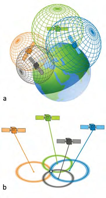
operations, freeing them up for other tasks as well as Force Base in Colorado. The system is young, relatively
reducing human errors. speaking. The GPS project was started in 1973, and the
first NAVigation System with Timing and Ranging (NAV-
Overview and History of the Global STAR) satellite was launched in 1978. The 24-satellite
Positioning System system became fully operational in 1995. A photograph
The GPS is owned by the US Government and is operated of a modern GPS-III satellite and a depiction of the satel-
and maintained by the US Air Force out of Shriever Air lite constellation are shown in Figure 1.
A precursor to the GPS, the Transit System, was designed
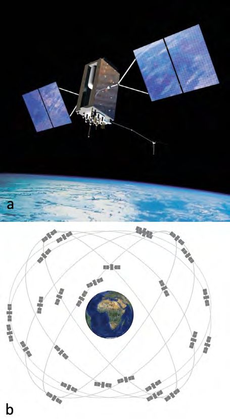
Figure 1. a: Image of Global Positioning System (GPS) III specifically to provide accurate location information to
satellite. A GPS III satellite is roughly the size of a small US Navy Polaris nuclear submarines and became the first
car and orbits approximately 20,200 km above the earth. operational satellite navigation system in 1964 (Guier and
b: Configuration of satellite constellation. The original Weiffenbach, 1998). There is not enough space here to go
constellation contained 6 orbitals with slots for 4 satellites into all of the science and technology advances that paved
each, and only 24 satellites are required to operate at any the way for the modern GPS, including the satellite geod-
given time. But, in 2011, this was expanded to accommodate esy work of Gladys Mae West (featured in Shetterly, 2016,
additional satellites to improve coverage. Source: United and the movie Hidden Figures), but the gps.gov website,
States Government (available at gps.gov/multimedia/images). maintained by the national coordination office for space-
based positioning, navigation, and timing and hosted by
the National Oceanic and Atmospheric Administration
(NOAA) has a wealth of useful information and links.
The US-based GPS satellites are not the only navigational
satellites orbiting the earth. Indeed, a Russian-based
GLObal NAVigation Satellite System (GLONASS)
became operational around the same time as the GPS.
The United States and Russia both started construction
of their own GNSS constellations at the height of the
Cold War. More recently, in June 2020, China launched
the final satellite in the third generation of the BeiDou
Navigation Satellite System, which now provides world-
wide coverage. Europe has launched Galileo, which has
been operational since 2019, and the complete 30-satel-
lite system is expected by the time you read this article.
Galileo is the only purely civilian system; the systems
launched by the United States, China, and Russia are all
at least partially owned or operated by the military. Most
modern smartphones have the capability to receive sig-
nals from multiple constellations.
How Does the Global Positioning
System Work?
GPS satellites continuously broadcast electromagnetic
signals that travel through the atmosphere, providing
their location and precise timing information. (I refer to
the GPS, but this can be applied more globally to other
GNSS constellations as they operate using the same
principles.) A GPS satellite transmits multiple signals,
Spring 2021 • Acoustics Today 53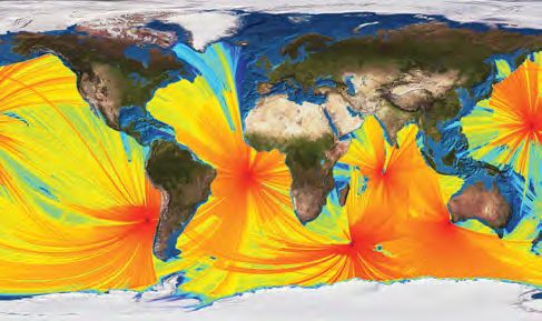
UNDERWATER GPS

                                                                         where c is the speed of light (299,792,458 m/s) and t is the
                                                                         time of flight for the signal traveling through space. This
                                                                         time of flight is the difference between the time the signal is
                                                                         broadcast by the satellite and the time the signal is received.
                                                                         Once a GPS receiver obtains the distance between itself
                                                                         and at least four satellites, it can use geometry to deter-
                                                                         mine its location and simultaneously correct its time.

                                                                         The concept is relatively simple and is demonstrated in
                                                                         Figure 2. If we know just the range from a single satel-
                                                                         lite, the location of the receiver could be anywhere on an
                                                                         imaginary sphere with the satellite located at its center.
                                                                         Combining the ranges received from 4 satellites, along
                                                                         with precise timing information, provides a single inter-
                                                                         section point in 3-dimensional space that corresponds
                                                                         to the position of the GPS receiver. This is referred to as
                                                                         trilateration (often confused with triangulation, which
                                                                         involves measuring angles rather than distances).

                                                                         Apparent from Eq. 1, an inaccurate estimate of the signal
                                                                         travel time will give an incorrect distance from receiver
                                                                         to satellite and therefore an inaccurate position. Precise
                                                                         timing is therefore vital to GPS operation. Nanosec-
                                                                         onds in timing error on the satellites lead to meters of
                                                                         positioning error on the ground. Each satellite has an
 Figure 2. a: Depiction of positioning of a GPS receiver using           atomic clock onboard, which provides precise timing
 trilateration in three dimensions. Each sphere with a satellite         information. These precise clocks are updated twice a day
 at its center represents the distance calculated from Eq. 1. The        to correct the clock’s natural drift using an even higher
 four spheres intersect at the location of the GPS receiver. b:          precision atomic clock based on land.
 Trilateration with four satellites projected onto two dimensions
 with the single point of intersection determining the location of the   Underwater Positioning and Navigation
 GPS receiver. Presented with permission from gisgeography.com.          Using Acoustics
                                                             It is interesting to note that satellite navigation systems
                                                             were first designed with submarines in mind even though
including ranging signals and navigation messages. The the GPS is not useful beneath the sea surface. Electro-
original GPS design contained two ranging signals: a magnetic waves from the satellites travel very efficiently
coarse/acquisition (C/A) code and a restricted precision through the atmosphere but are quickly attenuated
(P) code reserved for military and government applica- underwater. Underwater vehicles and underwater instru-
tions. Each satellite transmits a C/A code with a carrier mentation are therefore unable to take full advantage of
frequency of 1,575.42 MHz. Galileo and BeiDou also the GPS infrastructure.
transmit signals at this carrier frequency, which is in the
microwave band, outside of the visible spectrum.             Submarines do take advantage of underwater acous-
                                                             tic signals, and the field of underwater acoustics has
The time that it takes the signal to reach the receiver is largely been driven by military applications (Muir and
used to calculate a range or distance (d) from the satellite Bradley, 2016). Acoustic waves are mechanical pres-
with the following simple relationship                       sure waves and therefore do not propagate well in the
                                                             (near) vacuum of space but travel more efficiently
                           d=c×t               (         1) and more quickly in denser media. Because of this,

54   Acoustics Today • Spring 2021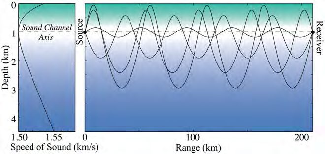
sound travels faster in seawater than in air and it is         These buoys have constant access to GPS positioning so
less quickly attenuated.                                       they do not require a survey.

The same basic relationship from Eq. 1 that is used to         Short-baseline (SBL) systems operate on a smaller scale,
calculate the distance from satellites can be applied to       and the SBL transducers are typically fixed to a surface
acoustic signals as well. Here, rather than multiplying the    vessel. Ultrashort-baseline (USBL) systems are typically
time that the GPS signal has traveled by the speed of light,   a small transducer array, also often fixed to a surface
the travel time of the signal is multiplied by the speed of    vehicle, which use phase (arrival angle) information of
sound in the medium through which it is traveling. The         the acoustic signals to determine the vehicle position.
speed of sound in the ocean is roughly 1,500 m/s. This is
much slower than the speed of light, and it is also quite      These types of acoustic localization work in a similar way
variable because the speed of sound in seawater depends        to GPS localization, with electromagnetic waves; how-
on the seawater temperature, salinity, and depth.              ever, they all operate in relatively small regions. Note that
                                                               these acoustic-positioning methods have been described
Traditional Underwater Positioning and                         in the context of underwater vehicles, but they can be
Local Vehicle Navigation Systems                               used for other purposes as well, including tracking drift-
Underwater vehicles routinely get position and timing          ing instrumentation or even animals underwater.
from a GPS receiver when they are at the surface, but
once they start to descend, this is no longer available.       Long-Range Underwater Acoustics
Vehicles navigate underwater using some combination of      Propagation in the SOFAR Channel
dead reckoning, vehicle hydrodynamic models, inertial       Attenuation of acoustic signals in the ocean is highly
navigation systems (INSs), and local navigation networks    dependent on frequency. The signals commonly used
(Paull et al., 2014). Positioning in the z direction, the   for LBL, SBL, and USBL localization networks typi-
depth in the ocean, is straightforward with a pressure      cally have frequencies of tens of kilohertz and upward.
sensor, which can reduce the dimensionality of the prob-    These signals may travel for a few kilometers, but lower
lem to horizontal positioning in x and y, or longitude and  frequency signals on the order of hundreds of hertz or
latitude, respectively.                                     lower are capable of traveling across entire ocean basins
                                                            underwater. This was demonstrated in 1991 by the Heard
Dead reckoning estimates the position using a known Island Feasibility Test, where a signal was transmitted
starting point that is updated with measurements of vehi- from Heard Island in the Southern Indian Ocean and
cle speed and heading as time progresses. Larger vehicles, received at listening stations across the globe, from Ber-
such as submarines, may have an onboard INS that inte- muda in the Atlantic Ocean to Monterey, CA, in the
grates measurements of acceleration to estimate velocity Eastern Pacific Ocean (Munk et al., 1994).
and thereby position. These measurements are, however,
subject to large integration drift errors.                  Refractive effects of the ocean waveguide are usually
                                                            taken into account when using the acoustic-positioning
Because of the need for more position accuracy than methods described above because an acoustic arrival
afforded by the submarine systems discussed above, it often does not take a direct path from the source to the
comes as no surprise that underwater vehicles also use receiver, and often a number of arrivals resulting from
acoustics for localization. A long-baseline (LBL) acoustic- multiple propagation paths are received. The refractive
positioning system is composed of a network of acoustic effects of the ocean waveguide become even more impor-
transponders, often fixed on the seafloor with their posi- tant as ranges increase. Acoustic arrivals can be spread
tions accurately surveyed. The range measurements from out over several seconds; however, the time arrival struc-
multiple transponders are used to determine position. ture can be predicted based on the sound speed profile.
LBL systems typically operate on scales of 100 meters to
several kilometers and have accuracies on the order of a The speed of sound in the ocean increases with increasing
meter. Transponder buoys at the surface can also provide hydrostatic pressure (depth in the ocean) and with higher
positioning accuracy similar to a seafloor LBL network. temperatures that occur near the surface. This leads to

                                                                                         Spring 2021 • Acoustics Today   55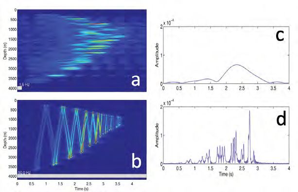
UNDERWATER GPS

a sound speed minimum referred to as the sound chan-         for ocean temperature. Each ray has traveled a unique
nel axis, which exists at approximately 1,000 m depth,       path through the ocean and therefore carries with it
although the depth can vary depending on where you           information on the sound speed along the particular path
are on the globe (Figure 3).                                 that it has traveled. On a very basic level, we are looking
                                                             again at the relationship from Eq. 1, but here distance and
The SOFAR channel, short for SOund Fixing And Rang- travel time are known, and we are inverting for sound
ing, refers to a sound propagation channel (Worzel et speed, which is a proxy for temperature. In ocean acous-
al., 1948) that is centered around the sound channel axis. tic tomography, the variability in these acoustic travel
Sound from an acoustic source placed at the sound speed times is measured regularly over a long period of time
minimum will be refracted by the sound speed profile, (acoustic sources and receivers often remain deployed
preventing low-angle energy from interacting with the in the ocean for a year at a time) to track how the ocean
lossy seafloor and enabling the sound rays to travel for temperature is changing. This method was described by
very long distances, up to thousands of kilometers.          Worcester et al. (2005) in the very first issue of Acoustics
                                                             Today and more thoroughly in the book, Ocean Acoustic
The rays take different paths when traveling over these Tomography, by Munk et al. (1995).
long ranges, as seen in Figure 3. The arrival time at a
receiver is an integrated measurement of travel time The variability in these travel times is measured in mil-
along the path of the ray. Rays that are launched at angles liseconds; therefore, as with a GNSS, the acoustic travel
near the horizontal stay very close to the sound speed time measurements must be extremely precise. Great care
minimum. Rays that are launched at higher angles travel is taken to use clocks with low drift rates and to correct
through the upper ocean and deep ocean, and although for any measured clock drift at the end of an experiment.
they take a longer route than the lower angle rays, they
travel through regions of the ocean that have a faster The locations of the acoustic sources and receivers also
sound speed and therefore arrive at a receiver before their must be accurate because inaccuracies in either position
counterparts that took the shorter, slower road.             would lead to an inaccurate calculation of distance, which
                                                             would impact the inversion for sound speed based on the
Ocean Acoustic Tomography Measurements                       simple relationship of Eq. 1. The sources and receivers
Ocean acoustic tomography takes advantage of the vari- used in typical ocean acoustic tomography applications
ability in measured travel times for specific rays to invert are on subsurface ocean moorings, meaning that there

 Figure 3. Left: canonical profile of sound speed as a function of depth in the ocean (solid line). Right: refracted acoustic ray paths
 from a source at 1,000 m depth to a receiver at 1,000 m depth and at a range of 210 km. The Sound Channel Axis (dashed line) is
 located at the sound speed minimum at a depth of 1 km. Adapted by Discovery of Sound in the Sea (see dosits.org) from Munk et
 al., 1995, Figure 1.1, reproduced with permission.

56   Acoustics Today • Spring 2021
is an anchor on the seafloor with a wire stretched up to a RAFOS sources have been useful to track floats in open
buoy that sits below the surface to hold the line taut. The water, but when there is sea ice present and the float is
sources and hydrophone receivers are mounted on this unable to get to the surface for a GPS position, underwater
line. Additional floatation is also mounted on the line positioning becomes even more important. A recent study
to keep the mooring standing upright, but it is subject in the Weddell Gyre near Antarctica tracked 22 floats
to ocean currents, so it moves around in a watch circle under ice that were unable to surface to obtain position
about the anchor position. An instrument at the top of a from the GPS for eight months (Chamberlain et al., 2018).
5,000-m mooring could be swept several hundred meters
from the latitude and longitude position of the anchor by Similar to RAFOS, a separate long-range navigation
ocean currents. A LBL array of acoustic transponders, as system in the Arctic used surface buoys to transmit
described in Traditional Underwater Positioning and GPS positions to floats and vehicles for under-ice rang-
Local Vehicle Navigation Systems, is typically deployed ing, with an accuracy of 40 m over 400-km ranges. This
around each mooring position to track the motion of system operated at 900 Hz, with a programmable band-
the sources and receivers throughout the experiment to width from 25 to 100 Hz (Freitag et al., 2015).
correct for the changes in distance between the sources
and receivers. RAFOS signals have a bandwidth of 1.6 Hz and there-
fore less time resolution than a more broadband source.
Positioning with Long-Range Underwater Figure 4, a and b, contrast predictions of the arrival
Acoustic Measurements structure at a 1,145-km range for a RAFOS source with
The same core concepts of inferring distance from mea- a broadband source having a bandwidth of 50 Hz. In
surements of signal travel time that we see in GNSS both cases, the latest arriving energy is concentrated near
and local underwater acoustic networks can also apply the depth of the sound channel axis, corresponding to
at long ranges. Neutrally buoyant oceanographic floats rays that stayed at depths with low sound speeds. The
called swallow floats were equipped with acoustic ping- early arrivals are from rays that ventured into the higher
ers to be tracked by a nearby ship; these were adapted speed regions of the sound speed profile (in Figure 3,
to take advantage of the deep sound channel and were dark blue and green) and therefore also span more of the
subsequently known as SOFAR floats. The first SOFAR ocean depth. In both cases, we can see that the energy is
float was deployed in 1968 and was detected 846 km away spread over about 4 s, but the broadband source provides
(Rossby and Webb, 1970). better resolution.
The SOFAR float signals were originally received by the Figure 4, c and d, shows slices of these acoustic predic-
SOund SUrveillance System (SOSUS) of listening stations tions at a 2,000 m depth. The broadband signal shown
operated by the US military. This system tracked more in Figure 4d exhibits sharp peaks in the arrival that can
than just floats and enemy submarines. It also received be identified with individual ray paths.
acoustic signals from earthquakes, and there is a wonder-
ful 43-day record of passively tracking of an individual The increased bandwidth is one of the design suggestions
blue whale, nicknamed Ol’ Blue, as it took 3,200-km tour for a potential joint navigation/thermometry system
of the North Atlantic Ocean (Nishimura, 1994). addressed in Duda et al. (2006). A system of sources is
suggested with center frequencies on the order of 100-
The existing listening system was convenient, but 200 Hz and a 50-Hz bandwidth.
equipping each float with an acoustic source was tech-
nologically challenging and expensive. In the 1980s, the The acoustic sources used for ocean acoustic tomography
concept was flipped so that the float had the hydrophone applications are broadband sources designed to trans-
receiver, and acoustic sources transmitted to the floats mit over ocean basin scales. A 2010-2011 ocean acoustic
from known locations to estimate range to the float. tomography experiment performed in the Philippine Sea
The name was also flipped, and the floats are known as featured six acoustic sources in a pentagon arrangement
RAFOS, an anadrome for SOFAR (Rossby et al., 1986). and provided a rich dataset for evaluating long-range
Spring 2021 • Acoustics Today 57UNDERWATER GPS
positioning algorithms. The sources used in this particu- How Feasible Is a Global Navigation
lar experiment had a center frequency of about 250 Hz Acoustic System?
and a bandwidth of 100 Hz. Because acoustic signals are able to propagate over extremely
long ranges underwater, acoustics could provide an under-
The sources were used to localize autonomous underwater water analogue to the electromagnetic GNSS signals that
vehicles that had access to a GPS at the sea surface but only are used for positioning in the land, air, and space domains.
surfaced a few times a day. Hydrophones on the vehicles There are definite differences between using an underwater
received acoustic transmissions from the moored sources acoustic positioning system and a GNSS, however. GNSS
at ranges up to 700 km, and these signals were used to esti- satellites orbit the earth twice a day and transmit continu-
mate the position of the vehicle when it was underwater ously. Acoustic sources do not need to be in orbit, but proper
(Van Uffelen et al., 2013). The measured acoustic arrivals placement of the sources would enable propagation to most
were similar to the modeled arrival shown in Figure 4d. regions in the oceans of the world.
The measurements of these peaks collected on the vehicle
were matched to predicted ray arrivals to determine range. The far reach of underwater acoustic propagation is dem-
This method takes advantage of the multipath arrivals onstrated by the International Monitoring System (IMS)
in addition to signal travel time. As with other acoustic operated by the Comprehensive Nuclear Test Ban Treaty
methods and with the GPS, ranges from multiple sources Organization (CTBTO). The IMS monitors the globe for
were combined to obtain estimates of vehicle position. The acoustic signatures of nuclear tests with only six under-
resulting positions had estimated uncertainties less than water passive acoustic hydrophone monitoring stations
100 m root mean square (Van Uffelen et al., 2015). worldwide. Figure 5 shows the coverage of these few sta-
tions. Signals received on these hydroacoustic stations
Other long-range acoustic-ranging methods incorporate pre- were used to localize an Argentinian submarine that was
dictions of acoustic arrivals based on ocean state estimates lost in 2017 using acoustic recordings of the explosion
(Wu et al., 2019). An algorithm introduced by Mikhalevsky on IMS listening stations at ranges of 6,000 and 8,000 km
et al. (2020) provides a “cold start’ capability that does not from the site (Dall’Osto, 2019).
require an initial estimate of the acoustic arrival and has
positioning orders on the order of 60 m. These results were You may note that Figure 5 does not show much coverage
validated using hydrophone data with known positions that in the Arctic Ocean and that the sound speed structure is
received the Philippine Sea source signals. As with the afore- quite different at high latitudes because it does not have
mentioned method, this algorithm relies on the travel-time the warm surface that we see in Figure 3; however, long-
resolution afforded by the broadband source signals. range propagation has been demonstrated in the Arctic
Figure 4. Predictions of the acoustic arrival
for a 260-Hz source at a range of 1,145 km. for
a RAFOS source with a bandwidth of 1.6 Hz
(a) and for a source with a bandwidth of 50
Hz (b). The arrivals in both cases are spread
over about 4 s, with early arriving energy from
higher angle rays and later arriving energy
from rays launched at low angles that stayed
near the depth of the sound channel axis. Slices
of the plots shown in a and b were taken at
a depth of 2,000 m for the RAFOS source
(c) and broadband source (d) to contrast the
travel time resolution. Adapted from Duda et
al., 2006, with permission.
58 Acoustics Today • Spring 2021a multipurpose acoustic observing system (Howe et al.,
2019), would transmit this information as well to enable
mobile platform positioning and navigation. Such a
system could also provide ocean acoustic tomography
measurements and passive acoustic monitoring for bio-
logical, natural, and anthropogenic sources.
Final Thoughts
The GPS satellite constellation was originally designed
to meet national defense, homeland security, civil, com-
mercial, and scientific needs in the air, in the sea, and on
Figure 5. Global coverage of the Comprehensive Nuclear land. The age of artificial intelligence and big data has
Test Ban Treaty Organization (CTBTO) International made GPS data on land incredibly useful to all of us in
Monitoring System (IMS), shown by a 3-dimensional model our everyday life. Not only can we use information on
of low-frequency (UNDERWATER GPS
Freitag, L., Ball, K., Partan, J., Koski, P., and Singh, S. (2015). Long
range acoustic communications and navigation in the Arctic. Pro- About the Author
ceedings of OCEANS 2015-MTS/IEEE, Washington, DC, October
19-22, 2015, pp. 1-5.
Lora J. Van Uffelen
Guier, W. H., and Weiffenbach, G. C. (1998). Genesis of satellite navi-
loravu@uri.edu
gation. Johns Hopkins APL Technical Digest 19(1), 14-17.
Heaney, K. D., and Eller, A. I. (2019). Global soundscapes: Parabolic equation Department of Ocean Engineering
modeling and the CTBTO observing system. The Journal of the Acoustical University of Rhode Island
Society of America 146(4) 2848. https://doi.org/10.1121/1.5136881. Narragansett, Rhode Island 02882,
Howe, B. M., Miksis-Olds, J., Rehm, E., Sagen, H., Worcester, P. F., and USA
Haralabus, G. (2019). Observing the oceans acoustically. Frontiers in Lora J. Van Uffelen is an assistant pro-
Marine Science 6, 426. https://doi.org/10.3389/fmars.2019.00426.
fessor in the Department of Ocean Engineering, University of
Mikhalevsky, P. N., Sperry, B. J., Woolfe, K. F., Dzieciuch, M. A.,
Rhode Island (Narragansett), where she teaches undergradu-
and Worcester, P. F. (2020). Deep ocean long range underwater
ate and graduate courses in underwater acoustics and leads
navigation, The Journal of the Acoustical Society of America 147(4),
the Ocean Platforms, Experiments, and Research in Acoustics
2365-2382. https://doi.org/10.1121/10.0001081.
(OPERA) Lab. She earned her PhD in oceanography from the
Muir, T. G., and Bradley, D. L. (2016). Underwater acoustics: A brief his-
Scripps Institution of Oceanography, University of California,
torical overview through World War II. Acoustics Today 12(2), 40-48.
San Diego (La Jolla). Her current research projects focus on
Munk, W., Worcester, P., and Wunsch, C. (1995). Ocean Acoustic
long-range underwater acoustic propagation, Arctic acous-
Tomography. Cambridge University Press, New York, NY.
tics, vehicle and marine mammal localization, and acoustic
Munk, W. H., Spindel, R. C., Baggeroer, A., and Birdsall, T. G. (1994).
sensing on underwater vehicles. She has participated in more
The Heard Island Feasibility Test. The Journal of the Acoustical Society
than 20 research cruises, with over 400 days at sea.
of America 96, 2330-2342.
Nishimura, C. E. (1994). Monitoring whales and earthquakes by using
SOSUS. 1994 Naval Research Laboratory Review, pp. 91-101.
Paull, L., Saeedi, S., Seto, M., and Li, H. (2014). AUV navigation and local-
ization: A review. IEEE Journal of Oceanic Engineering 39, 131-149. The Journal of the Acoustical
Rossby, T., and Webb, D. (1970). Observing abyssal motions by tracking Swal-
low floats in the SOFAR channel. Deep Sea Research and Oceanographic Society of America
Abstracts 17(2), 359-365. https://doi.org/10.1016/0011-7471(70)90027-6.
Rossby, T., Dorson, D., and Fontaine, J. (1986). The RAFOS system.
Journal of Atmospheric and Oceanic Technology 3, 672-679. Reflections
Shetterly, M. L. (2016). Hidden Figures: The American Dream and the
Untold Story of the Black Women Mathematicians Who Helped Win Don’t miss Reflections, The Journal of the
the Space Race. William Morrow, New York, NY. Acoustical Society of America’s series that
Van Uffelen, L. J., Howe, B. M. Nosal, E. M. Carter, G. S., Worcester, P. takes a look back on historical articles that
F., and Dzieciuch, M. A. (2015). Localization and subsurface position
error estimation of gliders using broadband acoustic signals at long have had a significant impact on the
range. Journal of Oceanic Engineering 41(3) 501-508. science and practice of acoustics.
https://doi.org/10.1109/joe.2015.2479016.
Van Uffelen, L. J., Nosal, E. M., Howe, B. M., Carter, G. S., Worcester,
P. F., Dzieciuch, M. A., Heaney, K. D., Campbell, R. L., and Cross, P.
S.. (2013). Estimating uncertainty in subsurface glider position using
transmissions from fixed acoustic tomography sources. The Journal
of the Acoustical Society of America 134, 3260-3271.
https://doi.org/10.1121/1.4818841.
Worcester, P. F., Dzieciuch M. A., and Sagen, H. (2020). Ocean acous-
tics in the rapidly changing Arctic. Acoustics Today 16(1), 55-64.
Worcester, P. F., Munk, W. H., and Spindel, R. C. (2005). Acoustic
remote sensing of ocean gyres. Acoustics Today 1(1), 11-17.
Worzel, J. L., Ewing, M., and Pekeris, C. L. (1948). Propagation of Sound
in the Ocean. Geological Society of America Memoirs 27, Geological
Society of America, New York, NY. https://doi.org/10.1130/MEM27.
Wu, M., Barmin, M. P., Andrew, R. K., Weichman, P. B., White, A. W., See these articles at:
Lavely, E. M., Dzieciuch, M. A., Mercer, J. A., Worcester, P. F., and acousticstoday.org/forums-reflections
Ritzwoller, M. H. (2019). Deep water acoustic range estimation based
on an ocean general circulation model: Application to PhilSea10
data. The Journal of the Acoustical Society of America 146(6), 4754-
4773. https://doi.org/10.1121/1.5138606.
60 Acoustics Today • Spring 2021You can also read


