Generating Seamless Global Daily AMSR2 Soil Moisture (SGD-SM) Long-term Products 2013-2019 - ESSD
←
→
Page content transcription
If your browser does not render page correctly, please read the page content below
Generating Seamless Global Daily AMSR2 Soil Moisture (SGD-SM)
     Long-term Products 2013-2019
     Qiang Zhang1 , Qiangqiang Yuan2, 3 * , Jie Li2 , Yuan Wang2 , Fujun Sun4 , and Liangpei Zhang1 *
     1
       State Key Laboratory of Information Engineering, Survey Mapping and Remote Sensing, Wuhan University, China
     2
       School of Geodesy and Geomatics, Wuhan University, China
     3
       Key Laboratory of Geospace Environment and Geodesy, Ministry of Education, Wuhan University, China
     4
       Beijing Electro-mechanical Engineering Institute, Beijing, China
     Correspondence: Qiangqiang Yuan (yqiang86@gmail.com) and Liangpei Zhang (zlp62@whu.edu.cn)

     Abstract. High quality and long-term soil moisture products are significant for hydrologic monitoring and agricultural man-
     agement. However, the acquired daily Advanced Microwave Scanning Radiometer 2 (AMSR2) soil moisture products are
     incomplete in global land (just about 30%∼80% coverage ratio), due to the satellite orbit coverage and the limitations of
     soil moisture retrieving algorithms. To solve this inevitable problem, we develop a novel spatio-temporal partial convolutional
5    neural network (CNN) for AMSR2 soil moisture products gap-filling. Through the proposed framework, we generate the seam-
     less global daily (SGD) AMSR2 soil moisture long-term products from 2013 to 2019. To further validate the effectiveness of
     these products, three verification ways are used as follows: 1) In-situ validation; 2) Time-series validation; And 3) simulated
     missing regions validation. Results show that the seamless global daily soil moisture products have reliable cooperativity with
     the selected in-situ values. The evaluation indexes of the reconstructed (original) dataset are correlation coefficient (R): 0.683
10   (0.687), Root Mean Squard Error (RMSE): 0.099 (0.095), and Mean Absolute Error (MAE): 0.081 (0.078), respectively. The
     temporal consistency of the reconstructed daily soil moisture products is ensured with the original time-series distribution of
     valid values. The spatial continuity of the reconstructed regions accords with the spatial information (R: 0.963∼0.974, RMSE:
     0.065∼0.073, and MAE: 0.044∼0.052). This dataset can be downloaded at https://doi.org/10.5281/zenodo.4417458 (Zhang
     et al., 2021).

15   1    Introduction

         Surface soil moisture is a crucial Earth land characteristic in describing hydrologic cycle system (Wigneron et al., 2003;
     Lievens et al., 2015). It can be applied for monitoring droughts and floods in agriculture (Samaniego et al., 2018) and geologic
     hazards (Long et al., 2014). To obtain the global and high-frequency soil moisture products, many active or passive satellite
     sensors have been launched such as Advanced Microwave Scanning Radiometer for EOS (AMSR-E), Advanced Microwave
20   Scanning Radiometer 2 (AMSR2), Soil Moisture Active and Passive (SMAP), Soil Moisture and Ocean Salinity (SMOS) and
     so on (McColl et al., 2017; Ma et al., 2019). Nevertheless, the acquired daily soil moisture products are always incomplete
     in global land (about 30%∼80% missing ratio in AMSR2), because of the satellite orbit coverage and the limitations of soil
     moisture retrieving algorithms (Cho et al., 2017; Long et al., 2019). The invalid land regions refer to the gap or information

                                                                     1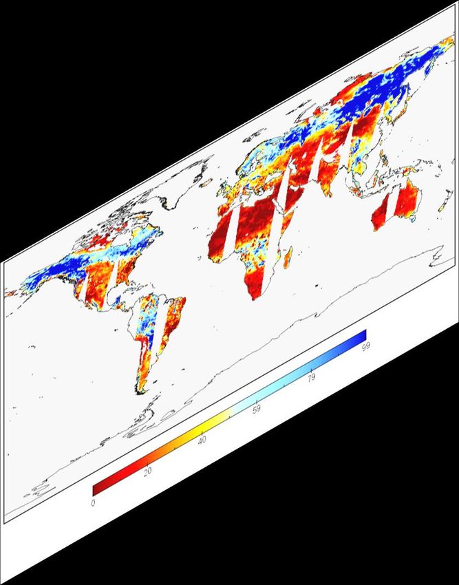
missing area. Especially in the regions close to the equator, or in the permafrost region, the soil moisture data missing degree
25   is more serious (Zeng et al., 2015; Santi et al., 2018). This phenomenon greatly disturbs subsequent soil moisture applications,
     especially for the consecutive daily temporal analysis and global spatial-distribution comparisons (Colliander et al., 2017; Liu
     et al, 2019).
       To reduce this negative effect, most existing works employed the strategy of multi-temporal soil moisture data selecting,
     multi-temporal soil moisture data averaging, or multi-temporal soil moisture data synthesizing. Detailed descriptions and anal-
30   yses of these three strategies (Bitar et al., 2017) are presented as follows:
       1) Multi-temporal soil moisture data selecting: Criterion of this strategy denotes to selecting the highest coverage regions
     in single date from multi-temporal soil moisture products (Wang and Qu, 2009). However, this assumption can only deal with
     local regions, and not applicable for global regions. The main reason is that almost all the global daily soil moisture products
     suffer from the defect of satellite orbit coverage missing and retrieving algorithm failure. Multi-temporal soil moisture data
35   selecting strategy greatly reduces the data utilization, and is not qualified for dense time-series analysis on daily temporal
     resolution (Liu et al., 2020; Purdy et al., 2018).
       2) Multi-temporal soil moisture data averaging: This strategy is commonly used for most soil moisture study or appli-
     cations. The incomplete soil moisture products are overall averaged as the monthly/quarterly/yearly results to generate the
     complete products (Jalilvand et al., 2019). For most applications and spatial analysis, this operation can effectively improve the
40   spatial soil moisture coverage (Zhao et al., 2020). However, it distinctly sacrifices the high-frequency temporal resolution as
     low-frequency temporal resolution, which also severely reduces the data utilization. In addition, it ignores the unique spatial-
     distribution of single day and loses the dense time-series changing information. In other word, the monthly/quarterly/yearly
     soil moisture data averaging operations damage the initial information on both spatial and temporal dimension.
       3) Multi-temporal soil moisture data synthesizing: Different from soil moisture data selecting and averaging, this strategy
45   employs the time-series daily soil moisture data and selects the valid observed value from corresponding time-series pixels.
     This strategy can produce synthesizing result through valid single-point, while it ignores the spatial local correlation and exists
     incontinuous and inconsistent effects in local regions. In addition, it also sacrifices high temporal resolution just as multi-
     temporal data averaging strategy (Peng et al., 2017; Sun et al., 2020).
       To overcome above-mentioned limitations, some missing values reconstruction methods have been developed especially
50   on multi-temporal images thick cloud removal and deadline gap-filling (Zhang et al., 2020a). For example, Zhu et al. (2011)
     proposed the multi-temporal neighboring homologous value padding method for thick cloud removal. Chen et al. (2011)
     presented an effective interpolating algorithm for recovering the invalid regions in Landsat images. Zhang et al. (2018a) built
     an integrative spatio-temporal-spectral network for missing data reconstruction in multiple tasks.
       In terms of the soil moisture products gap-filling, several methods have also been proposed to address this issue. Wang et al.
55   (2012) presented a penalized least square regression-based approach for global satellite soil moisture gap filling observation.
     Fang et al. (2017) introduced a long short-term memory network to generate spatial complete overlay SMAP in U.S. Long et
     al. (2019) fused multi-resolution soil moisture products, which can produce daily fine-resolution data in local regions. Llamas

                                                                      2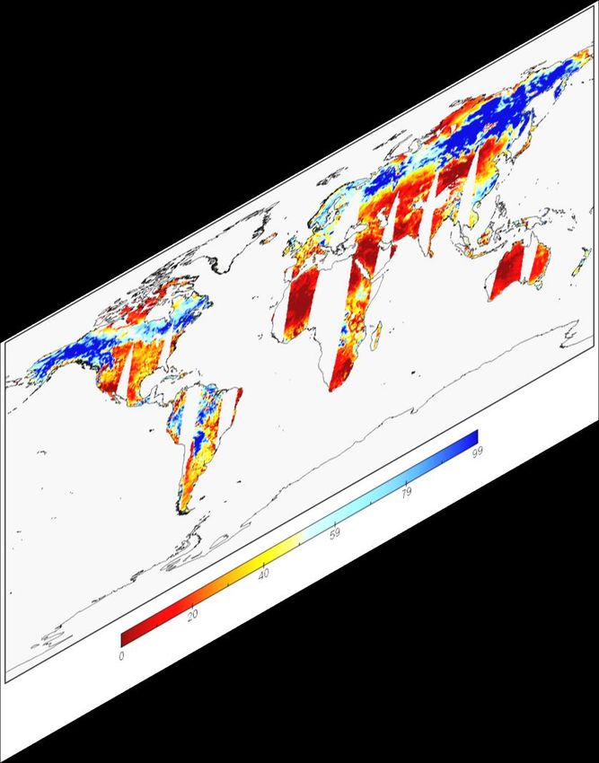
et al. (2020) used geostatistical techniques and multiple regression strategy to get spatial complete results of satellite-derived
     products. Overall, there are few works for soil moisture productions reconstructing on global and daily scale.
60       In spatial dimension, the invalid land areas and adjacent valid land areas exist the spatial consistency and spatial correlation
     on daily soil moisture products (Long et al., 2020). In temporal dimension, daily time-series changing curve of the same point
     natively appears with the continuous and smooth peculiarities (Chan et al., 2018). Overall, these methods can effectively fill
     the gaps of soil moisture products. However, these methods cannot simultaneously take both spatial and temporal information
     into consideration. In addition, the daily soil moisture products in global scale have not been exploited up to now.
65       Therefore, how about simultaneously extracting both spatial and temporal features for seamless global daily soil moisture
     products gap-filling? Recently, deep learning has gradually revealed the potential for remote sensing products processing
     (Chen et al., 2021). In consideration of the powerful feature expression ability via deep learning, can we utilize spatio-temporal
     information to generate long-term soil moisture products?
         From these perspectives, a novel spatio-temporal deep learning framework is proposed for global daily AMSR2 soil moisture
70   products gap-filling. By means of the proposed method, we can effectively break through the above-mentioned limitations. And
     finally, this work generates the seamless global daily AMSR2 soil moisture long-term products from 2013 to 2019. The main
     innovations are summarized as below:
         1) We develop a deep 3D partial reconstruing model, which can take both the spatial and temporal information into consid-
     eration. Aiming at the invalid or coastline region boundary, the 3D partial CNN and global-local loss function are presented
75   for better extracting the valid region features and ignoring the invalid regions through both soil moisture data and mask infor-
     mation.
         2) A seamless global daily (SGD) AMSR2 soil moisture long-term (2013-2019) dataset is generated through the proposed
     model. The dataset includes the original and reconstructing soil moisture data. And this SGD products could be directly
     downloaded at https://doi.org/10.5281/zenodo.4417458 (Zhang et al., 2021).
80       3) Three verification strategies are employed to testify the precision of our SGD soil moisture dataset as follows: in-situ
     validation; time-series validation; and simulated missing regions validation. Evaluating indexes demonstrate that the seamless
     global daily AMSR2 soil moisture dataset shows high accuracy, reliability, and robustness.
         The schema of this work is listed below. Sect 2 describes the study ASMR2 soil moisture products and in-situ soil moisture
     network data. Sect 3 presents the methodology for generating the seamless global daily AMSR2 soil moisture products. Sect
85   4 gives the experimental results and related validation results. The comparisons between time-series averaging method and
     proposed method are discussed in Sect 5. And at last, Sect 6 makes the conclusions of this study.

     2     Data description

     2.1    AMSR2 soil moisture products

         In consideration of the global coverage, temporal-resolution, and current availability, we select AMSR2 soil moisture prod-
90   ucts as the focused object. This sensor was onboard on the Global Change Observation Mission 1-Water (GCOM-W1) satellite,

                                                                       3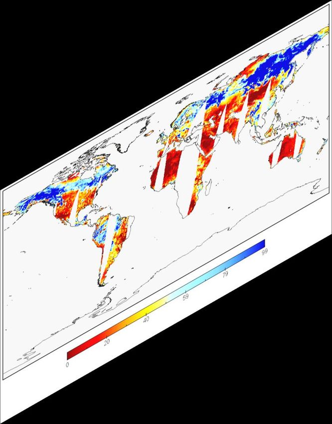
launched in May 2012 (Kim et al., 2015). The released datasets include three passive microwave band frequencies: 6.9 GHz
      (C1 band), 7.3 GHz (C2 band, new frequency compared with AMSR-E), and 10.7 GHz (X band). It can observe the global
      land two times within a day (Wu et al., 2016): ascending (day-time) and descending (night-time, about 0:00-1:00 AM of the
      local time) orbits. The primary spatial resolution of this datasets denotes 0.25◦ global grids. And the AMSR2 soil moisture
95    retrieval algorithms include Land Parameter Retrieval Model (LPRM) and Japan Aerospace Exploration Agency (JAXA) (Du
      et al., 2017; Kim et al., 2018). The error of soil moisture for each frequency were also given in AMSR2 products.
        In our study, we choose LPRM AMSR2 descending level 3 (L3) global daily 0.25◦ soil moisture products as the study
      data. To avoid introducing additional error and uncertainty, we didn’t carry out the downscaling operation of the generated
      SGD-SM products. This dataset was obtained from https://hydro1.gesdisc.eosdis.nasa.gov/. For instance, the original AMSR2
100   0.25◦ soil moisture data in April 2, 2019 is displayed in Fig. 1(a). Due to the satellite orbit coverage and limitations of soil
      moisture retrieving algorithms in tundra areas (Muzalevskiy et al., 2020), the acquired AMSR2 daily soil moisture products
      are always incomplete in global land (about 30%∼80% invalid ratio, excluding Antarctica and most of Greenland), as shown
      in Fig. 1(a). The daily global land coverage ratio of AMSR2 soil moisture data in 2019 is listed in Fig. 2. Distinctly, the global
      land coverage ratio is low in wintertime, and high in summertime. The mean global land coverage ratio in 2019 is just about
105   56.5% in AMSR2 soil moisture daily products. Apparently, these incomplete soil moisture data cannot be directly applied for
      subsequent spatial and time-series analysis, as mentioned in previous Sect 1.

            (a) Original global AMSR2 0.25◦ soil moisture data in April 2, 2019        (b) The spatial distribution of the used in-situ sites.

      Figure 1. AMSR2 soil moisture product and selected in-situ soil moisture sites

      2.2    International Soil Moisture Network in-situ data

        The International Soil Moisture Network (ISMN) was established from 2009 to now (Dorigo et al., 2011) providing the
      correction/validation schemes for remote sensing satellite-based soil moisture retrieval. ISMN includes the globally distributed
110   in-situ soil moisture sites supported by the earth observation of the European Space Agency (ESA) and many voluntary con-
      tributions of researchers and organizations from all over the world (Dorigo et al., 2012; Dorigo et al., 2013).

                                                                                  4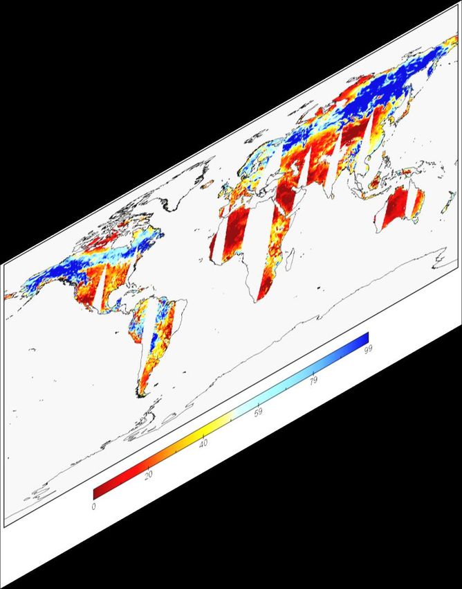
                                *OREDO/DQG&RYHUDJH5DWLR


                                                                                                                       0HDQ&RYHUDJH5DWLR


                                                                                                                                'D\

      Figure 2. The daily global land coverage ratio of AMSR2 soil moisture products in 2019

          The ISMN in-situ surface soil moisture values could be acquired through https://ismn.geo.tuwien.ac.at. In our experiments,
      we selected a portion of in-situ soil moisture sites of ISMN as ground truth values (Zhang et al., 2017), to testify the precision
      and credibility of the reconstructing datasets in Sect 4.2. The spatial distribution of the used in-situ sites is depicted in Fig.
115   1(b). It should be noted that the time range is restrained from 2013.1.1 to 2019.12.31. Then the daily soil moisture values are
      matched with the in-situ sites in the same location. Two neighboring in-situ hourly values are averaged as the ultimate result of
      current date (Dong et al., 2020).

      3    Methodology

          The flowchart of the presented framework is depicted in Fig. 3. The overall structure could be divided as two stages: the
120   training procedure and testing procedure. Firstly, we designate the processing daily soil moisture data in date T, and simultane-
      ously select its adjacent time-series data before and after four days (date T-4 to T+4). The corresponding land masks of these
      daily soil moisture data are generated through the invalid pixel marking.
          In the training procedure, these spatio-temporal soil moisture data and land mask patch groups are imported as the training
      data of the presented spatio-temporal 3-D reconstructing model through patch selecting and mask simulating. The convergence
125   condition denotes that the loss of the proposed model gradually decreases, and finally maintains smooth in training procedure
      through back-propagation (BP) in Fig. 3. Then in the testing procedure, seamless global daily reconstructing soil moisture
      data is outputted through the convergent model. Subsequently, the next processing daily soil moisture data is designated and
      repeat above-mentioned steps, until all the daily data are serially reconstructed in order. Details of the reconstructing model
      and network are described below.

                                                                                                                               5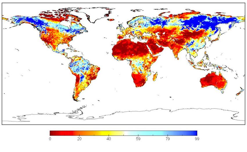
Training Procedure              Global Daily Soil Moisture Productions                Testing Procedure

              9-days Continuous Data                                                                 9-days Continuous Data
                 (Date: T-4 to T+4)                    Time-series                                      (Date: T-4 to T+4)
                                                       …
                                                       T-2
            Land Mask          Land Masks              T-1                                        Land Mask           Land Masks
             in T-day         in T-4 to T+4             T                                          in T-day          in T-4 to T+4
                                                       T+1
                                                       T+2
                               (exclude T)              …                                                               (exclude T)
                Patch
               Selecting
                                                                 Original

                                                                                                                                  T=T+1
               Spatio-temporal Patch
                                                                                                       Spatio-temporal 3-D
              Groups (Data and Masks)
                                                                                                       reconstructing model
                Mask
                                                       Time-series
              Simulating
                                                       …                                                 Seamless Soil
                 Spatio-temporal 3-D                   T-2                                              Moisture of T-day
                 reconstructing model                  T-1
                                                        T                                                                        No
                                         Yes           T+1                                                    Finish?
                    Convergence?                       T+2
                           No                           …                                                          Yes
            BP        Model                                                                                 Time-series
                    Optimization                              Reconstructed                                 Productions

      Figure 3. Flowchart of the presented framework

130   3.1    Spatio-temporal 3-D reconstructing model

        The spatio-temporal soil moisture reconstructing model is displayed in Fig. 4. After assigning the original soil moisture
      data in date T, time-series soil moisture data and corresponding masks in date T-4 to T+4 are simultaneously imported as the
      3D-tensor inputs of the presented deep reconstructing model in Fig. 4. In spatial dimension, missing and non-missing areas
      exist the spatial consistency in daily soil moisture data. In temporal dimension, the daily time-series changing curve of the
135   same point natively appears with the continuous and smooth peculiarities. Therefore, the 3D CNN is employed to process the
      spatio-temporal soil moisture data in this model. Through this way, we can jointly utilize both spatial and temporal information
      of these time-series soil moisture products. Further, it can better richly exploit the deep spatio- temporal feature for data
      reconstructing and model optimization. The structure and details are depicted in Fig. 4.
        This network includes 11 layers (3D partial CNN unit and ReLU (Rectified Linear Unit)) in Fig. 4. The size of 3D filters is
140   all set as 3×3×3. Number of feature maps before ten layers is fixed as 90, and the channel of feature map in the final layer is

                                                                     6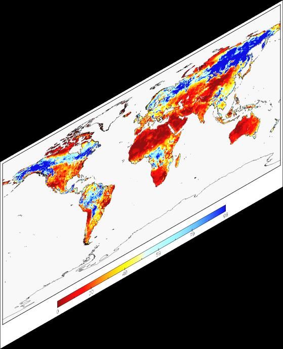
exported as 1. It should be noted that after finishing each partial 3D-CNN layer, we must update all the new masks for next
layer. The mask updating operation is defined in Sect 3.2. In terms of the model training and optimization, three steps: patch
selecting, mask simulating, and back propagation are performed in Sect 3.3. For network optimization, we take the global loss
and local loss into consideration. As described in Fig. 3, this deep reconstructing model need to be learned with large training
145 label samples, before the testing procedure for outputting global seamless daily soil moisture products. The global land mask
and the mask in current date T are also employed for the global loss and local loss in Fig. 4. Descriptions of partial 3D-CNN
and model optimization are demonstrated in Sect 3.2 and Sect 3.3, respectively.
Time-series SM in
Date T-4 to T+4
SM in Date T Global Land Mask
Layer 1 Layer 2 Layer 3 … Layer 10
3×3×3×90 3×3×3×90 3×3×3×90 3×3×3×90
s=1 s=1 s=1 s=1
Layer 11
Global Loss
… +
Local Loss
3×3×3×1
3D Partial 3D Partial 3D Partial 3D Partial
CNN + ReLU CNN + ReLU CNN + ReLU CNN + ReLU s=1
Updating Updating Updating
Mask in Date T Masks Masks Masks Mask in Date T
Time-series Masks
in Date T-4 to T+4
Figure 4. Spatio-temporal soil moisture 3D reconstructing model
3.2 Partial convolutional neural network
Deep convolution neural network has been widely applied for nature image reconstructing (Liu et al., 2018a; Yeh et al., 2017;
150 Liu et al., 2019) and satellite imagery recovering (Yuan et al., 2019; Zhang et al., 2019; Zhang et al., 2020b). Nevertheless, it
should be highlighted that the valid and invalid pixels simultaneously exist especially around the coast regions and gap regions
(Pathak et al., 2016). The common CNN ignores the location information of invalid or valid pixels in soil moisture data, which
cannot eliminate the invalid information (Liu et al., 2018b). Therefore, to solve this negative effect, we develop the partial
3D-CNN to ignore the invalid information in the proposed reconstructing model.
155 Before introducing the partial convolution, the operation of common convolution in most deep learning framework can be
defined as below:
x = WT X + b (1)
7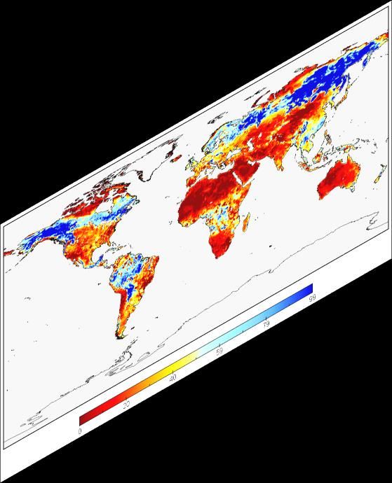
where X denotes the inputted tensor data. W and b are the weight and bias parameters, respectively. Different from the common
convolution, the mask information M of the corresponding soil moisture data is introduced into the partial convolution:
k1(w,h,t) k1
WT (X(w,h,t) M(w,h,t) ) + b, M(w,h,t) 6= 0
160 x0 = kM(w,h,t) k1 1
(2)
0, otherwise
where stands for the pixel-wise multiplication. w, h, and t refer to the width, height, and temporal number of the input data,
respectively. 1 denotes the identical dimension tensor with mask M, whose elements are all value 1. Obviously, the partial
convolutional output x0 is only decided by the valid soil moisture pixels of input X, rather than the invalid soil moisture pixels.
Through the mask M, we can effectively exclude the interference information of invalid soil moisture pixels such as marine
165 regions and gap regions. Then the scaling divisor in Eq. (2) further adjusts for the variational number of valid soil moisture
pixels.
After finishing each partial convolution layer, all the masks need to updated through the following rule: If the partial con-
volution can generate at least one valid value of the output result, then we mark this location as valid value in the new masks.
This updating operation is demonstrated as below:
Land
(w,h) · 1, M(w,h,t) 6= 0
170 m0 (w,h,t) = 1 (3)
0, otherwise
where Land(w,h) is the global land mask in location (w, h) of the global soil moisture product. This global land mask covers
six continents and excludes Antarctica and most of Greenland.
3.3 Model training and optimization
As shown in Fig. 3, the training procedure needs to generate large numbers of training samples for learning the proposed
175 spatio-temporal 3-D reconstructing model in Fig. 4. Different from the testing procedure, the training procedure additionally
contains the patch selecting, mask simulating, and back propagation (BP) steps. These three steps are significant for model
training and optimization. The purpose of patch selecting and mask simulating step in Fig. 3 is to establish the label (complete)-
data (incomplete) training samples in the deep learning framework. The significance of BP step in Fig. 3 is to optimize the
reconstructing network in Fig. 4 and acquire the loss convergence model for testing use.
180 In the patch selecting step, we traverse the global regions in date T to select the complete soil moisture patch label, whose
local land regions are undamaged. It should be noted the rest incomplete patches in date T are excluded because they cannot
participate in the supervised learning. The corresponding time-series soil moisture patches of this selected patch between date
T-4 to T+4, is set as the spatio-temporal 3D data patch groups. And their corresponding masks between date T-4 to T+4 is set
as the spatio-temporal 3D mask patch groups. After traversing the original global daily AMSR2 soil moisture products from
185 2013 to 2019, we finally establish the spatio-temporal data and mask patch groups with the number of 276488 patches. The
soil moisture patch size is fixed as 40×40 for patch selecting.
8
In the mask simulating step, 10000 patch masks of the size 40×40 are chosen from the global AMSR2 soil moisture masks
      from 2013 to 2019. The missing ratio range of these masks is set as [0.3, 0.7]. Then these patch masks are randomly selected
      for label patches use within the spatio-temporal data and mask patch groups. The complete patch in date T (label) is simulated
190   as the incomplete patch (data) through the above mask. And the original corresponding mask of this patch needs also to be
      replaced. After traversing and building the label-data 3D spatio-temporal patch groups, this dataset is set as the training samples
      for the usage of reconstructing network in Fig. 3.
        In the back propagation step, we need a loss function to iteratively optimal the learning parameters of the deep reconstructing
      network. This operation follows the chain rule in model optimizing. The Euclidean loss function is employed in most data
195   reconstruction or regression issues based on deep learning, such as satellite products downscaling (Fang et al., 2020) and
      retrieving (Lee et al., 2019). Nevertheless, Euclidean loss function only pays attention to the holistic information bias for
      network optimization. It ignores the soil moisture particularity of the local areas, especially in local coastal, mountain, and
      hinterland regions. However, this particularity is extremely significant for invalid regions gap-filling, because of the spatial
      heterogeneity in soil moisture products. Therefore, to take both the global consistency and local soil moisture particularity into
200   consideration, the global land mask and current mask in date T are both employed after the final layer as shown in Fig. 3.
      Further, the reconstructing network presents the local and global 2-norm loss as below:

                                                   2
      ζlocal = k(1 − MT )     (SMrec − SMori )k2                                                                                     (4)

                                              2
      ζglobal = kMG      (SMrec − SMori )k2                                                                                          (5)

205   where MT stands for current mask patch in date T. MG represents the corresponding global land mask patch. SMrec and
      SMori denote the reconstructed soil moisture patch and original seamless soil moisture patch, respectively. The unified loss
      function of the reconstructing network combines ζlocal and ζglobal as below:

      ζ(Θ) = ζlocal + η · ζglobal                                                                                                    (6)

      where Θ refers to the learnable arguments for each layer of the deep reconstructing model. η denotes the balancing factor to
210   adjust the ζlocal and ζglobal . In this work, we fixed this factor as 0.1 during the training procedure.
        After building up this unified loss function, the presented reconstructing model employs Adam algorithm as the gradient
      descent strategy. The number of batch size in this model is fixed as 128 for network training (Shi et al., 2020). The total epochs
      and initial learning rate are determined as 300 and 0.001, respectively. Starting every 30 epochs, the learning rate is degraded
      through decay coefficient 0.5 (Zhang et al., 2018b). The training and testing procedure of the proposed model are implemented
215   by Pytorch platform. The software environment is listed as follows: Python 3.7.4 language, Windows 10 operating system, and

                                                                        9
PyCharm 2019 integrated development environment (IDE). The final soil moisture products are exported as hierarchical data
format, which both contains the original and reconstructed soil moisture data.
4 Experimental results and validation
In this section, we provide the experimental results and related validation results to testify the availability of the presented
220 framework. Through this framework, we finally generate the seamless global daily AMSR2 soil moisture long-term products
from 2013.1.1 to 2019.12.31. The daily soil mositure products are saved as NetCDF4 format. It should be highlighted that this
dataset can be directly downloaded at https://doi.org/10.5281/zenodo.4417458 (Zhang et al., 2021) for free-use. An example
Python code of extracting this dataset are also available at https://github.com/qzhang95/SGD-SM.
We firstly give two sample seamless reconstructing results of global time-series soil moisture products. The original and
225 reconstructed results are both given for comparisons. Later, to further validate the effectiveness of these products, three verifi-
cation ways are respectively employed as follows:
1) In-situ validation.
2) Time-series validation.
3) Simulated missing regions validation.
230 In-situ validation is utilized to compare the reconstructed soil moisture with original AMSR2 soil moisture through the
selected in situ sites from the spatial prospect. In-situ shallow-depth soil moisture sites can be employed as the ground-truth
to validate the reconstructing satellite soil moisture products. Time-series validation is employed for evaluating the time-series
continuity from the temporal prospect. Soil moisture time-series scatters can obviously reveal the annual periodic variations
for time-series validation. Simulated missing regions validation is used to testify the soil moisture consistency from the spatial
235 prospect. It can verify the spatial consistency between the valid and invalid soil moisture regions.
4.1 Experimental results
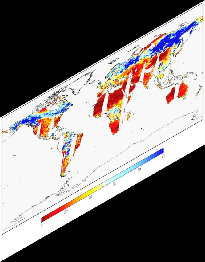
As displayed in Fig. 5 (a)-(h) and Fig. 6 (a)-(h), original and reconstructing global daily time-series AMSR2 soil moisture
products between 2019.6.1 to 6.4 and 2016.10.1 to 10.4 are given as the sample results, respectively. The left column lists
the original incomplete soil moisture results, and the right column lists the corresponding complete soil moisture results after
240 reconstructed by the proposed method in 2019.6.1 to 6.4 and 2016.10.1 to 10.4. We ignore the coverage of Antarctica and most
of Greenland, because the satellite soil moisture data within these regions behaves perennially missing.
From the spatial dimension, the reconstructing global soil moisture products are consistent between invalid regions and their
adjacent valid regions in Fig. 5 and Fig. 6. Especially around the high-value areas and low-value areas, the spatial information
consecutive without obvious reconstructing boundary effects such as in Africa, Australia, and Europe in Fig. 5 and Fig. 6.
245 From the temporal dimension, although the incomplete time-series daily results are highly similar and correlative, there
are still some variations and differences between each other. The proposed method performs well on consistent temporal
information preserving and specific temporal information predicting in Fig. 5 and Fig. 6.
10(a) Original SM in 2019.6.1 (b) Reconstructing SM in 2019.6.1
(c) Original SM in 2019.6.2 (d) Reconstructing SM in 2019.6.2
(e) Original SM in 2019.6.3 (f) Reconstructing SM in 2019.6.3
(g) Original SM in 2019.6.4 (h) Reconstructing SM in 2019.6.4
Figure 5. Original/reconstructing global daily SM results between 2019.6.1 to 6.4
11(a) Original SM in 2016.10.1 (b) Reconstructing SM in 2016.10.1
(c) Original SM in 2016.10.2 (d) Reconstructing SM in 2016.10.2
(e) Original SM in 2016.10.3 (f) Reconstructing SM in 2016.10.3
(g) Original SM in 2016.10.4 (h) Reconstructing SM in 2016.10.4
Figure 6. Original/reconstructing global daily SM results between 2016.10.1 to 10.4
124.2 In-situ validation
In-situ shallow-depth soil moisture sites can be employed as the ground-truth to validate the reconstructing satellite soil
250 moisture products. We select 125 soil moisture stations (0-10cm) through ISMN between 2013.1.1 to 2019.12.31. Nine soil
moisture in-situ sites and the corresponding reconstructing data within invalid regions are then contrast as the scatter plots in
Fig. 7 (a)-(i), respectively. The horizontal axis stands for in-situ soil moisture value. Meanwhile the vertical axis represents
reconstructing soil moisture value. It should be highlighted that due to the lacks of part recorded data between 2013 to 2019,
most in-situ values are incompleteness with different point numbers. As shown in Fig. 7 (a)-(i), the correlation coefficients (R)
255 indexes are distributed between 0.679 to 0.754. The root-mean-square error (RMSE) and mean absolute error (MAE) indexes
are distributed from 0.026 to 0.134 and from 0.021 to 0.107, respectively.
100 100 100
R=0.726 R=0.679 R=0.707
Reconstructed SM value (percent)
Reconstructed SM value (percent)
Reconstructed SM value (percent)
RMSE=0.059 m 3 /m3 RMSE=0.134 m 3 /m3 RMSE=0.04 m 3 /m3
80 MAE=0.047 m 3 /m3 80 MAE=0.107 m 3 /m3 80 MAE=0.032 m 3 /m3
60 60 60
40 40 40
20 20 20
0 0 0
0 20 40 60 80 100 0 20 40 60 80 100 0 20 40 60 80 100
In-situ SM value (percent) In-situ SM value (percent) In-situ SM value (percent)
(a) COSMOS-026 (b) COSMOS-055 (c) COSMOS-098
100 100 100
R=0.699 R=0.685 R=0.754
Reconstructed SM value (percent)
Reconstructed SM value (percent)
Reconstructed SM value (percent)
RMSE=0.074 m 3 /m3 RMSE=0.035 m 3 /m3 RMSE=0.026 m 3 /m3
80 MAE=0.058 m 3 /m3 80 MAE=0.028 m 3 /m3 80 MAE=0.021 m 3 /m3
60 60 60
40 40 40
20 20 20
0 0 0
0 20 40 60 80 100 0 20 40 60 80 100 0 20 40 60 80 100
In-situ SM value (percent) In-situ SM value (percent) In-situ SM value (percent)
(d) COSMOS-044 (e) COSMOS-033 (f) COSMOS-076
100 100 100
R=0.689 R=0.725 R=0.691
Reconstructed SM value (percent)
Reconstructed SM value (percent)
Reconstructed SM value (percent)
RMSE=0.027 m 3 /m3 RMSE=0.039 m 3 /m3 RMSE=0.079 m 3 /m3
80 MAE=0.021 m 3 /m3 80 MAE=0.031 m 3 /m3 80 MAE=0.063 m 3 /m3
60 60 60
40 40 40
20 20 20
0 0 0
0 20 40 60 80 100 0 20 40 60 80 100 0 20 40 60 80 100
In-situ SM value (percent) In-situ SM value (percent) In-situ SM value (percent)
(g) COSMOS-087 (h) COSMOS-048 (i) COSMOS-012
Figure 7. Scatters of the in-situ/reconstructed soil moisture values within selected stations
13In additions, we compare the reconstructed with original AMSR2 soil moisture products through the selected 125 in-situ
sites, as listed in Table 1. The averaged R, RMSE, and MAE of the original and reconstructed soil moisture products are
0.683 (0.687), 0.099 (0.095), and 0.081 (0.078), respectively. Overall, the accuracy of reconstructed soil moisture products
260 is generally accorded with the original products. The differences of these indexes R, RMSE and MAE are minor between the
original and reconstructed soil moisture results in Table 1. To some degree, this validation ensures the reliability and availability
of the proposed seamless global daily AMSR2 soil moisture products.
Table 1. Comparisons between original and reconstructed soil moisture products
Evaluation index
Soil Moisture products
R RMSE MAE
Original 0.687 0.095 0.078
Reconstructed 0.683 0.099 0.081
4.3 Time-series validation
To further validate the reconstructed soil moisture results, time-series variations of both original and reconstructed re-
265 sults are stacked in six points around the six continents: Africa (0.375◦ N, 36.875◦ E), Europe (49.375◦ N, 35.125◦ E), Asia
(38.125◦ N, 117.375◦ E), North America (39.875◦ N, 106.125◦ W), South America (15.125◦ S, 52.625◦ W), Australia (30.125◦ S,
150.375◦ E), respectively. As described in Fig. 8(a)-(f), the horizontal axis stands for daily time-series date between Jan 1 2013
to Dec 31 2019. The vertical axis represents the soil moisture value. The blue points refer to the original valid soil moisture
daily results, and the red forks stands for the reconstructed invalid soil moisture daily results in Fig. 8.
270 As depicted in Fig. 8(a)-(f), most of the soil moisture time-series scatters can obviously reveal the annual periodic variations.
The reconstructed soil moisture results generally behave fine temporal consistency with the original soil moisture results in
different areas. Related low soil moisture values mostly existed in the droughty season of winter with the frozen lands such as
in Fig. 8(d). Related high soil moisture values mainly generated in the moist season of summer with more rainy days, especially
in Fig. 8 (b), (d) and (f).
275 Overall, compared with the whole original variation tendency between 2013 to 2019, the generated seamless global daily
AMSR2 soil moisture long-term products can steadily reflect the temporal consistency and variation. It is significant for time-
series applications and analysis. This daily time-series validation also demonstrates the robustness of the presented method and
the availability of the established seamless global daily products.
1490 Original
Reconstructed
SM (percent)
60
30
0
2013 2014 2015 2016 2017 2018 2019
(a) Time-series results in Africa (0.375◦ N, 36.875◦ E)
90 Original
Reconstructed
SM (percent)
60
30
0
2013 2014 2015 2016 2017 2018 2019
(b) Time-series results in Europe (49.375◦ N, 35.125◦ E)
90 Original
Reconstructed
SM (percent)
60
30
0
2013 2014 2015 2016 2017 2018 2019
(c) Time-series results in Asia (38.125◦ N, 117.375◦ E)
90 Original
Reconstructed
SM (percent)
60
30
0
2013 2014 2015 2016 2017 2018 2019
(d) Time-series results in North America (39.875◦ N, 106.125◦ W)
90 Original
Reconstructed
SM (percent)
60
30
0
2013 2014 2015 2016 2017 2018 2019
(e) Time-series results in South America (15.125◦ S, 52.625◦ W)
90 Original
Reconstructed
SM (percent)
60
30
0
2013 2014 2015 2016 2017 2018 2019
(f) Time-series results in Australia (30.125◦ S, 150.375◦ E)
Figure 8. Original/reconstructed time-series results in selected regions
154.4 Simulated missing regions validation
280 In addition to the time-series consistency in Sect 4.3, the spatial continuity is also important for the reconstructed seamless
soil moisture products. Therefore, to further testify this key point, we carry out the simulated missing regions validation in this
subsection. Based on the original soil moisture products, six simulated square missing regions are performed in six continents,
respectively. Through thisway,we can easily compare the reconstructed SM regions with original SM regions, to validate
the 2D spatial continuity of the proposed SGD-SM products. We select four dates of the long-term soil moisture products:
285 2013.7.25, 2015.7.25, 2017.7.25, and 2019.7.25 as the simulated objects. For example, original and reconstructed results with
simulated missing regions in 2019.7.25 are depicted in Fig. 9(a) and (b), respectively. The simulated missing regions can be
clearly observed in Fig. 9(a) around the six continents. Detailed original and reconstructed spatial information of four simulated
patches in 2015.7.25 are displayed in Fig. 10. Table 2 gives the evaluation index (R, RMSE, MAE) of the simulated patches
between 2013 to 2019. Then the original-reconstructed scatters of simulated regions in 2013, 2015, 2017, and 2019.7.25 are
290 listed in Fig. 11(a)-(b), respectively.
As shown in Fig. 9 (a) and (b), the reconstructed invalid regions are consecutive between the original valid regions. And
in the simulated missing regions, the spatial texture information is also continuous without obvious boundary reconstructing
effects in Fig. 9(b). To better distinguish the spatial details of reconstructed soil moisture, we select four enlarged patches in
simulated regions in Fig. 10. It can be clearly observed that the reconstructed patches perform the high consistency with the
295 original patches, as displayed in Fig. 10.
In addition, the reconstructed soil moisture patches in simulated missing regions behave high reconstructing accuracy, whose
R values are distributed between 0.963 to 0.974 in Table 2 and Fig. 11(a)-(d). RMSE and MAE values also perform well on
0.065 to 0.073 m3 /m3 and 0.044 to 0.052 m3 /m3 in Table 2 and Fig. 11(a)-(d), respectively. Overall, this simulated missing
regions validation manifests the reconstructing ability of spatial information continuity.
Table 2. Evaluation indexes of the simulated patches between 2013 to 2019
Evaluation index
Year
R RMSE MAE
2013 0.974 0.065 0.044
2014 0.963 0.073 0.052
2015 0.968 0.069 0.050
2016 0.972 0.067 0.046
2017 0.966 0.070 0.049
2018 0.970 0.065 0.046
2019 0.969 0.069 0.048
Average 0.968 0.068 0.471
16(a) Original soil moisture result with simulated missing regions (square regions)
(b) Reconstructed soil moisture result
Figure 9. Original and reconstructed results with simulated missing regions in 2019.7.25
17Patch 1 Patch 2 Patch 3 Patch 4
Original
Reconstructed
Figure 10. Detailed original/reconstructed spatial information of four simulated patches in 2015.7.25
100 100
R=0.974 R=0.968
Reconstructed SM value (percent)
Reconstructed SM value (percent)
RMSE=0.065 m 3 /m3 RMSE=0.069 m 3 /m3
80 MAE=0.044 m 3 /m3 80 MAE=0.05 m3 /m3
60 60
40 40
20 20
0 0
0 20 40 60 80 100 0 20 40 60 80 100
Original SM value (percent) Original SM value (percent)
(a) Scatter of simulated regions in 2013.7.25 (b) Scatter of simulated regions in 2015.7.25
100 100
R=0.966 R=0.969
Reconstructed SM value (percent)
Reconstructed SM value (percent)
RMSE=0.07 m 3 /m3 RMSE=0.069 m 3 /m3
80 MAE=0.049 m 3 /m3 80 MAE=0.048 m 3 /m3
60 60
40 40
20 20
0 0
0 20 40 60 80 100 0 20 40 60 80 100
Original SM value (percent) Original SM value (percent)
(c) Scatter of simulated regions in 2017.7.25 (d) Scatter of simulated regions in 2019.7.25
Figure 11. Original-reconstructed scatter of simulated regions in 2013, 2015, 2017, and 2019.7.25
18300 5 Discussion
5.1 Comparisons with time-series averaging
As mentioned in Sect 1, some simple strategies such as time-series averaging can be also employed for synthesizing the
complete soil moisture products. Therefore, we perform the comparisons between the time-series averaging approach and the
presented method, to further validate the effectiveness and rationality of our dataset and framework. In terms of the time-series
305 averaging method, it averages the time-series daily soil moisture data to reconstruct gap regions. The original soil moisture
result, time-series averaging result, and the proposed reconstructing result in 2016.9.10 are shown in Fig. 12(a)-(c), respectively.
Three reconstructed regions are marked with black circle in Fig. 12(b) and (c). The evaluation index comparisons between the
time-series averaging method and proposed method are listed in Table 3 through the corresponding in-situ data validations.
(a) Original
(b) Time-series averaging (c) Proposed
Figure 12. Original/time-series averaging/proposed global soil moisture results in 2016.9.10
As displayed in the balck circled regions of Fig. 12(b) and (c), we can clearly distinguish the spatial discontinuity in the
310 time-series averaging result. Reversely, the proposed method performs better on spatial continuity between the valid and invalid
regions. The evaluation indexes R, RMSE, and MAE also manifest the superiority of the presented approach, compared with the
19Table 3. Evaluation index (R, RMSE, MAE) comparisons between the time-series averaging and proposed method
Evaluation index
Method
R RMSE MAE
Time-series averaging 0.635 0.124 0.093
Proposed 0.708 0.085 0.066
time-series averaging method in Table 3. The main reason is that daily soil moisture products exist temporal differences. While
the time-series averaging strategy cannot use the 2D-spatial information and ignores these temporal differences. Therefore, it
reflects the obvious “boundary difference effect” especially in the circled regions of Fig. 12(b). This also reveals the limitations
315 and shortages of the time-series averaging method. On the contrary, the proposed method jointly utilizes both spatial and
temporal information of these time-series soil moisture products. Further, it can better richly exploit the deep spatio-temporal
feature for soil moisture data reconstructing. Overall, this discussion demonstrates the superiority of the proposed framework
on time-series products daily reconstructing, especially compared with the time-series averaging strategy.
5.2 Uncertainty analyse of the SGD-SM products
320 Uncertainty analyse is important for remote sensing quantitative products. The uncertainties in this generated SGD-SM
product can be classified as three types: 1) The errors of original AMSR2 SM product; 2) The meteorological factors such
as precipitation and snowfall; 3) The generalization of proposed reconstructing model. Detailed descriptions of these three
uncertainties are listed as follows:
1) The errors of original AMSR2 SM product: The proposed SGD-SM product is generated based on original AMSR2
325 SM product. While this original AMSR2 SM product also exists errors, due to the satellite sensor imaging and SM retrieval
algorithm. As shown in Table 1, the R, RMSE, and MAE evaluation indexes of the original AMSR2 SM product are 0.687,
0.095, and 0.078, respectively. These errors are also inevitably transmitted into the generated SGD-SM product.
2) The meteorological factors: SGD-SM relies on the temporal continuity and spatial consistency for daily SM gap-filling.
Nevertheless, if the unusual meteorologic occurs in single day such as precipitation and snowfall, it may destroy above as-
330 sumption and influence the reconstructing effects. This uncertainty can be noticed in time-series validation, especially for rainy
season.
3) The generalization of proposed reconstructing model: In this work, we train the proposed network through selecting com-
plete soil moisture patches. In addition, the simulated masks are also chosen from the daily soil moisture products. However,
it still exists the differences between the training data and testing data, such as land covering type, mask size, and so on. This
335 uncertainty may disturb the generalization of proposed reconstructing model, to some degree.
206 Conclusions
In this work, aiming at the spatial incompleteness and temporal incontinuity, we generate a seamless global daily (SGD)
AMSR2 soil moisture long-term products from 2013 to 2019. To jointly utilize spatial and temporal information, a novel
spatio-temporal partial CNN is proposed for AMSR2 soil moisture products gap-filling. The partial 3D-CNN and global-local
340 loss function are developed for better extracting valid region features and ignoring invalid regions through data and mask
information. Three validation strategies are employed to testify the precision of our seamless global daily products as follows:
1) In-situ validation; 2) Time-series validation; And 3) simulated missing regions validation. Evaluating results demonstrate
that the seamless global daily AMSR2 soil moisture dataset shows high accuracy, reliability, and robustness.
Although the proposed framework performs well on generating this seamless global daily soil moisture dataset, some draw-
345 backs and limitations still need to be overcome especially on multi-source data fusion, spatio-temporal information extracting
and deep learning model optimization. In our future work, we will introduce multi-source information fusion into the proposed
model, such as precipitation and snowfall. The proposed reconstructing model will be increasingly improved by means of more
powerful units and structures. In addition, we will consider more soil moisture products in our future work such as AMSR-E,
SMOS-IC, SMAP and so on.
350 7 Data availability
This dataset can be downloaded at https://doi.org/10.5281/zenodo.4417458 (Zhang et al., 2021).
Author contributions. ZQ designed the proposed model and performed the experiments. YQQ and ZLP revised the whole manuscript. LJ,
WY, and SFJ provided related data and some figures of this work. All authors read and provided suggestions for this manuscript.
Competing interests. All authors proclaim that they have no conflict of interests.
355 Acknowledgements. We sincerely thank ISMN organization, for them supplying scientific sites data.
21References
Bitar, A., Mialon, A., Kerr, Y. H., et al. (2017). The global SMOS Level 3 daily soil moisture and brightness temperature maps. Earth
System Science Data, 9(1), 293-315.
360 Chan, S. K., Bindlish, R., O’Neill, P., Jackson, T., Njoku, E., Dunbar, S., Colliander, A. (2018). Development and assessment of the SMAP
enhanced passive soil moisture product. Remote Sensing of Environment, 204, 931-941.
Chen, J., Zhu, X., Vogelmann, J. E., Gao, F., Jin, S. (2011). A simple and effective method for filling gaps in Landsat ETM+ SLC-off
images. Remote Sensing of Environment, 115(4), 1053-1064.
Chen, Y., Feng, X., Fu, B. (2021). An improved global remote-sensing-based surface soil moisture (RSSSM) dataset covering 2003-2018.
365 Earth System Science Data, 13(1), 1-31
Cho, E., Su, C. H., Ryu, D., Kim, H., Choi, M. (2017). Does AMSR2 produce better soil moisture retrievals than AMSR-E over Australia?
Remote Sensing of Environment, 188, 95-105.
Colliander, A., Jackson, T. J., Bindlish, R., et al. (2017). Validation of SMAP surface soil moisture products with core validation sites.
Remote Sensing of Environment, 191, 215-231.
370 Dong, J., Crow, W. T., Tobin, K. J., et al. (2020). Comparison of microwave remote sensing and land surface modeling for surface soil
moisture climatology estimation. Remote Sensing of Environment, 242, 111756.
Dorigo, W., de Jeu, R., Chung, D., Parinussa, R., Liu, Y., Wagner, W., Fernández-Prieto, D. (2012). Evaluating global trends (1988–2010)
in harmonized multi-satellite surface soil moisture. Geophysical Research Letters, 39(18).
Dorigo, W.A., Wagner, W., Hohensinn, R., Hahn, S., Paulik, C., Xaver, A., Gruber, A., Drusch, M., Mecklenburg, S., van Oevelen,
375 P., Robock, A., Jackson, T. (2011). The International Soil Moisture Network: a data hosting facility for global in situ soil moisture
measurements. Hydrology and Earth System Sciences, 15, 1675–1698.
Dorigo, W.A., Xaver, A., Vreugdenhil, M., Gruber, A., Hegyiová, A., Sanchis-Dufau, A.D., Zamojski, D., Cordes, C., Wagner, W., Drusch,
M. (2013). Global automated quality control of in situ soil moisture data from the international soil moisture network. Vadose Zone J. 12.
Du, J., Kimball, J. S., Jones, L. A., Kim, Y., Glassy, J. M., Watts, J. D. (2017). A global satellite environmental data record derived from
380 AMSR-E and AMSR2 microwave Earth observations. Earth System Science Data, 9, 791.
Fang, K., Shen, C., Kifer, D., Yang, X. (2017). Prolongation of SMAP to spatiotemporally seamless coverage of continental US using a
deep learning neural network. Geophysical Research Letters, 44(21), 11-030.
22Fang, L., Zhan, X., Yin, J., et al. (2020). An Intercomparing Study of Algorithms for Downscaling SMAP Radiometer Soil Moisture
Retrievals. Journal of Hydrometeorology.
385 Jalilvand, E., Tajrishy, M., Hashemi, S. A. G. Z., Brocca, L. (2019). Quantification of irrigation water using remote sensing of soil moisture
in a semi-arid region. Remote Sensing of Environment, 231, 111226.
Kim, H., Parinussa, R., Konings, A. G., et al. (2018). Global-scale assessment and combination of SMAP with ASCAT (active) and
AMSR2 (passive) soil moisture products. Remote Sensing of Environment, 204, 260-275.
Kim, S., Liu, Y. Y., Johnson, F. M., Parinussa, R. M., Sharma, A. (2015). A global comparison of alternate AMSR2 soil moisture products:
390 Why do they differ? Remote Sensing of Environment, 161, 43-62.
Lee, C. S., Sohn, E., Park, J. D., Jang, J. D. (2019). Estimation of soil moisture using deep learning based on satellite data: a case study of
South Korea. GIScience and Remote Sensing, 56(1), 43-67.
Lievens, H., Tomer, S. K., Al Bitar, A., et al. (2015). SMOS soil moisture assimilation for improved hydrologic simulation in the Murray
Darling Basin, Australia. Remote Sensing of Environment, 168, 146-162.
395 Liu, G., Reda, F. A., Shih, K. J., Wang, T. C., Tao, A., Catanzaro, B. (2018a). Image inpainting for irregular holes using partial convolutions.
In Proceedings of the European Conference on Computer Vision (ECCV) (pp. 85-100).
Liu, G., Shih, K. J., Wang, T. C., Reda, F. A., Sapra, K., Yu, Z., Catanzaro, B. (2018b). Partial convolution based padding. arXiv preprint
arXiv:1811.11718.
Liu, H., Jiang, B., Xiao, Y., Yang, C. (2019). Coherent semantic attention for image inpainting. In Proceedings of the IEEE International
400 Conference on Computer Vision (pp. 4170-4179).
Liu, X., Huang, Y., Xu, X., Li, X., Li, X., Ciais, P., Zeng, Z. (2020). High-spatiotemporal-resolution mapping of global urban change from
1985 to 2015. Nature Sustainability, 1-7.
Liu, X., Pei, F., Wen, Y., Li, X., Wang, S., Wu, C., Liu, Z. (2019). Global urban expansion offsets climate-driven increases in terrestrial
net primary productivity. Nature communications, 10(1), 1-8.
405 Llamas, R. M., Guevara, M., Rorabaugh, D., Taufer, M., Vargas, R. (2020). Spatial Gap-Filling of ESA CCI Satellite-Derived Soil Moisture
Based on Geostatistical Techniques and Multiple Regression. Remote Sensing, 12(4), 665.
Long, D., Bai, L., Yan, L., et al. (2019). Generation of spatially complete and daily continuous surface soil moisture of high spatial
resolution. Remote Sensing of Environment, 233, 111364.
Long, D., Shen, Y., Sun, A., et al. (2014). Drought and flood monitoring for a large karst plateau in Southwest China using extended
410 GRACE data. Remote Sensing of Environment, 155, 145-160.
23Long, D., Yan, L., Bai, L., Zhang, C., Li, X., Lei, H., Yang, H., Tian, F., Zeng, C., Meng, X., Shi, C. (2020). Generation of MODIS-like
land surface temperatures under all-weather conditions based on a data fusion approach. Remote Sensing of Environment, 246, 111863
Ma, H., Zeng, J., Chen, N., et al. (2019). Satellite surface soil moisture from SMAP, SMOS, AMSR2 and ESA CCI: A comprehensive
assessment using global ground-based observations. Remote Sensing of Environment, 231, 111215.
415 McColl, K. A., Alemohammad, S. H., Akbar, R., et al. (2017). The global distribution and dynamics of surface soil moisture. Nature
Geoscience, 10(2), 100-104.
Muzalevskiy, K., Ruzicka, Z. (2020). Detection of soil freeze/thaw states in the Arctic region based on combined SMAP and AMSR-2
radio brightness observations. International Journal of Remote Sensing, 41(14), 5046-5061.
Pathak, D., Krahenbuhl, P., Donahue, J., Darrell, T., Efros, A. A. (2016). Context encoders: Feature learning by inpainting. In Proceedings
420 of the IEEE Conference on Computer Vision and Pattern Recognition (pp. 2536-2544).
Peng, J., Loew, A., Merlin, O., Verhoest, N. E. (2017). A review of spatial downscaling of satellite remotely sensed soil moisture. Reviews
of Geophysics, 55(2), 341-366.
Purdy, A. J., Fisher, J. B., Goulden, M. L., Colliander, A., Halverson, G., Tu, K., Famiglietti, J. S. (2018). SMAP soil moisture improves
global evapotranspiration. Remote Sensing of Environment, 219, 1-14.
425 Samaniego, L., Thober, S., Kumar, R., Wanders, N., Rakovec, O., Pan, M., Marx, A. (2018). Anthropogenic warming exacerbates European
soil moisture droughts. Nature Climate Change, 8(5), 421-426.
Santi, E., Paloscia, S., Pettinato, S., Brocca, L., Ciabatta, L., Entekhabi, D. (2018). On the synergy of SMAP, AMSR2 AND SENTINEL-1
for retrieving soil moisture. International Journal of Applied Earth Observation and Geoinformation, 65, 114-123.
Shi, Q., Liu, M., Liu, X., Liu, P., Zhang, P., Yang, J., Li, X. (2020). Domain adaption for fine-grained urban village extraction from satellite
430 images. IEEE Geoscience and Remote Sensing Letters, 17(8), 1430-1434.
Sun, Z., Long, D., Yang, W., Li, X., Pan, Y. (2020). Reconstruction of GRACE Data on Changes in Total Water Storage Over the Global
Land Surface and 60 Basins. Water Resources Research, 56(4), e2019WR026250.
Wang, G., Garcia, D., Liu, Y., De Jeu, R., Dolman, A. J. (2012). A three-dimensional gap filling method for large geophysical datasets:
Application to global satellite soil moisture observations. Environmental Modelling and Software, 30, 139-142.
435 Wang, L., Qu, J. (2009). Satellite remote sensing applications for surface soil moisture monitoring: A review. Frontiers of Earth Science
in China, 3(2), 237-247.
Wigneron, J. P., Calvet, J. C., Pellarin, T., Van de Griend, A. A., Berger, M., Ferrazzoli, P. (2003). Retrieving near-surface soil moisture
from microwave radiometric observations: current status and future plans. Remote Sensing of Environment, 85(4), 489-506.
24Wu, Q., Liu, H., Wang, L., Deng, C. (2016). Evaluation of AMSR2 soil moisture products over the contiguous United States using in situ
440 data from the International Soil Moisture Network. International Journal of Applied Earth Observation and Geoinformation, 45, 187-199.
Yeh, R. A., Chen, C., Yian Lim, T., Schwing, A. G., Hasegawa-Johnson, M., Do, M. N. (2017). Semantic image inpainting with deep
generative models. In Proceedings of the IEEE Conference on Computer Vision and Pattern Recognition (pp. 5485-5493).
Yuan, Q., Zhang, Q., Li, J., Shen, H., Zhang, L. (2019). Hyperspectral image denoising employing a spatial–spectral deep residual convo-
lutional neural network. IEEE Transactions on Geoscience and Remote Sensing, 57(2), 1205-1218.
445 Zeng, J., Li, Z., Chen, Q., Bi, H. Y., Qiu, J. X., Zou, P. F. (2015). Evaluation of remotely sensed and reanalysis soil moisture products over
the Tibetan Plateau using in-situ observations. Remote Sensing of Environment, 163, 91-110.
Zhang, Q., Yuan, Q., Li, J., Li, Z., Shen, H., Zhang, L. (2020a). Thick cloud and cloud shadow removal in multitemporal imagery using
progressively spatio-temporal patch group deep learning. ISPRS Journal of Photogrammetry and Remote Sensing, 162, 148-160.
Zhang, Q., Yuan, Q., Li, J., Liu, X., Shen, H., Zhang, L. (2019). Hybrid noise removal in hyperspectral imagery with a spatial–spectral
450 gradient network. IEEE Transactions on Geoscience and Remote Sensing, 57(10), 7317-7329.
Zhang, Q., Yuan, Q., Li, J., Sun, F., Zhang, L. (2020b). Deep spatio-spectral Bayesian posterior for hyperspectral image non-iid noise
removal. ISPRS Journal of Photogrammetry and Remote Sensing, 164, 125-137.
Zhang, Q., Yuan, Q., Zeng, C., Li, X., Wei, Y. (2018a). Missing data reconstruction in remote sensing image with a unified spatial-
temporal-spectral deep convolutional neural network. IEEE Transactions on Geoscience and Remote Sensing, 56(8), 4274-4288.
455 Zhang, Q., Yuan, Q., Li, J., Yang, Z., Ma, X. (2018b). Learning a dilated residual network for SAR image despeckling. Remote Sensing,
10(2), 196.
Zhang, Q., Yuan, Q., Li, J., Wang, Y., Sun, F., Zhang, L. (2021). SGD-SM: Generating Seamless Global Daily AMSR2 Soil Moisture
Long-term Products (2013-2019) (Version 1.0) [Data set]. Zenodo. DOI: 10.5281/zenodo.4417458.
Zhang, X., Zhang, T., Zhou, P., Shao, Y., Gao, S. (2017). Validation analysis of SMAP and AMSR2 soil moisture products over the United
460 States using ground-based measurements. Remote Sensing, 9(2), 104.
Zhao, T., Hu, L., Shi, J., et al. (2020). Soil moisture retrievals using L-band radiometry from variable angular ground-based and airborne
observations. Remote Sensing of Environment, 248, 111958.
Zhu, X., Gao, F., Liu, D., Chen, J. (2011). A modified neighborhood similar pixel interpolator approach for removing thick clouds in
Landsat images. IEEE Geoscience and Remote Sensing Letters, 9(3), 521-525.
25You can also read