Flexible Dataset Distillation: Learn Labels Instead of Images
←
→
Page content transcription
If your browser does not render page correctly, please read the page content below
Flexible Dataset Distillation: Learn Labels Instead of Images
                                                                          Ondrej Bohdal1 , Yongxin Yang1 , Timothy Hospedales1
                                                                                                 1
                                                                                               The University of Edinburgh
                                                                                  {ondrej.bohdal, yongxin.yang, t.hospedales}@ed.ac.uk
arXiv:2006.08572v2 [cs.LG] 21 Oct 2020

                                                                     Abstract                                  is largely specific to the architecture used to train it (thus
                                                                                                               preventing its use to accelerate neural architecture search
                                           We study the problem of dataset distillation – creating a small     – NAS, for example), and must use a highly-customized
                                           set of synthetic examples capable of training a good model.
                                                                                                               learner (a specific image visitation sequence, a specific se-
                                           In particular, we study the problem of label distillation – cre-
                                           ating synthetic labels for a small set of real images, and show     quence of carefully chosen meta-learned learning rates, and
                                           it to be more effective than the prior image-based approach         a specific number of learning steps). Altogether these con-
                                           to dataset distillation. Methodologically, we introduce a more      straints mean that existing distilled datasets are not general
                                           robust and flexible meta-learning algorithm for distillation,       purpose enough to be useful in practice, e.g. with off-the-
                                           as well as an effective first-order strategy based on convex        shelf learning algorithms. We propose a more flexible ap-
                                           optimization layers. Distilling labels with our new algorithm       proach to dataset distillation underpinned by both algorith-
                                           leads to improved results over prior image-based distillation.      mic improvements and changes to the problem definition.
                                           More importantly, it leads to clear improvements in flexibil-          Rather than creating synthetic images (Wang et al. 2018)
                                           ity of the distilled dataset in terms of compatibility with off-
                                           the-shelf optimizers and diverse neural architectures. Inter-
                                                                                                               for arbitrary labels, or a combination of synthetic images
                                           estingly, label distillation can also be applied across datasets,   and soft labels (Sucholutsky and Schonlau 2019), we fo-
                                           for example enabling learning Japanese character recognition        cus on crafting synthetic labels for arbitrarily chosen stan-
                                           by training only on synthetically labeled English letters.          dard images. Compared to these prior approaches focused
                                                                                                               on synthetic images, label distillation benefits from exploit-
                                                                                                               ing the data statistics of natural images and the lower-
                                                               1    Introduction                               dimensionality of labels compared to images as parameters
                                         Distillation is a topical area of neural network research             for meta-learning. Practically, this leads to improved perfor-
                                         that initially began with the goal of extracting the knowl-           mance compared to prior image distillation approaches. As
                                         edge of a large pre-trained model and compiling it into a             a byproduct, this enables a new kind of cross-dataset knowl-
                                         smaller model, while retaining similar performance (Hinton,           edge distillation (Figure 1). One can learn solely on a source
                                         Vinyals, and Dean 2014). The notion of distillation has since         dataset (such as English characters) with synthetic distilled
                                         found numerous applications and uses including the possi-             labels, and apply the learned model to recognise concepts
                                         bility of dataset distillation (Wang et al. 2018): extracting         in a disjoint target dataset (such as Japanese characters).
                                         the knowledge of a large dataset and compiling it into a small        Surprisingly, it turns out that models can make progress on
                                         set of carefully crafted examples, such that a model trained          learning to recognise Japanese only through exposure to En-
                                         on the small dataset alone achieves good performance. This            glish characters with synthetic labels.
                                         is of scientific interest as a tool to study neural network gen-         Methodologically, we define a new meta-learning algo-
                                         eralisation under small sample conditions. More practically,          rithm for distillation that does not require costly evaluation
                                         it has the potential to address the large and growing logis-          of multiple inner-loop (model-training) steps for each iter-
                                         tical and energy hurdle of neural network training, if ade-           ation of distillation. More importantly our algorithm leads
                                         quate neural networks can be quickly trained on small dis-            to a more flexible distilled dataset that is better transferable
                                         tilled datasets rather than massive raw datasets.                     across optimizers, architectures, learning iterations, etc. Fur-
                                             Nevertheless, progress towards the vision of dataset distil-      thermore, where existing dataset distillation algorithms rely
                                         lation has been limited as the performance of existing meth-          on second-order gradients, we introduce an alternative learn-
                                         ods (Wang et al. 2018; Sucholutsky and Schonlau 2019)                 ing strategy based on convex optimization layers that avoids
                                         trained from random initialization is far from that of full           high-order gradients and provides better optimization, thus
                                         dataset supervised learning. More fundamentally, existing             improving the quality of the distilled dataset.
                                         approaches are relatively inflexible in terms of the distilled           In summary, we contribute: (1) A dataset distillation
                                         data being over-fitted to the training conditions under which         method that produces flexible distilled datasets that exhibit
                                         it was generated. While there is some robustness to choice of         transferability across learning algorithms. This brings us
                                         initialization weights (Wang et al. 2018), the distilled dataset      one step closer to producing useful general-purpose dis-
Source: EMNIST                     Target: KMNIST                           methods select a relatively large part of the data (e.g. at least
                         Copy model
                                                                 True labels
                                                                               10%), while distillation extends down to using 10 images
                         Synthetic
                         labels                                                per category (≈ 0.2% of CIFAR-10 data) through example
                                                                               synthesis. We retain original data (like summarization meth-
             CNN                                  CNN                          ods), but synthesize labels (like distillation). This leads to
                                                                               a surprising observation – it is possible to synthesize labels
      Backprop:                                   Backprop:                    for a few fixed examples so a model trained on these exam-
      Model update                                Label update
                                                                               ples can directly (without any fine-tuning) solve a different
                                                                               problem with a different label space (Figure 1).
Figure 1: Label distillation enables training a model that can
classify Japanese characters after being trained only on En-                   Meta-Learning. Meta-learning algorithms can often be
glish letters and synthetic labels. Labels are updated only                    grouped (Hospedales et al. 2020) into offline approaches
during meta-training, after which a new model is trained.                      (e.g. Wang et al. (2018); Finn, Abbeel, and Levine (2017))
                                                                               that solve an inner optimization at every iteration of an
                                                                               outer optimization; and online approaches that solve the
tilled datasets. (2) Our distilled datasets can be used to train               base and meta-learning problem simultaneously (e.g. Balaji,
higher performance models than those prior work. (3) We                        Sankaranarayanan, and Chellappa (2018); Li et al. (2019)).
introduce the novel concept of cross-dataset distillation, and                 Meta-learning is related to hyperparameter optimization, for
demonstrate proofs of concept for this curiosity, such as                      example Maclaurin, Duvenaud, and Adams (2015); Lor-
English→Japanese letter recognition.                                           raine, Vicol, and Duvenaud (2020) efficiently unroll through
                                                                               many steps of optimization like offline meta-learning, while
                                                                               Luketina et al. (2016) optimize hyperparameters and the
                     2      Related Work                                       base model like online meta-learning. Online approaches are
Dataset Distillation. Most closely related to our work is                      typically faster, but optimize meta-parameters for a single
Dataset (Wang et al. 2018) and Soft-Label Dataset Dis-                         problem. Offline approaches are slower and typically limit
tillation (Sucholutsky and Schonlau 2019). They focus on                       the length of the inner optimization for tractability, but can
the problem of distilling a dataset or model (Micaelli and                     often find meta-parameters that solve a distribution of tasks
Storkey 2019) into a small number of example images,                           (as different tasks are drawn in each outer-loop iteration).
which are then used to train a new model. This can be seen                     In dataset distillation, the notion of ‘distribution over tasks’
as solving a meta-learning problem with respect to model’s                     corresponds to finding a dataset that can successfully train a
training data (Hospedales et al. 2020). The common ap-                         network in many settings, such as different initial conditions
proach is to initialise the distilled dataset randomly, use                    (Wang et al. 2018). Our distillation algorithm is a novel hy-
the distilled data to train a model, and then backpropagate                    brid of these two families. We efficiently solve the base and
through the model and its training updates to take gradient                    meta-tasks simultaneously as per the online approaches, and
steps on the dataset. Since the ‘inner’ model training algo-                   are thus able to use more inner-loop steps. However, we also
rithm is gradient-based, this leads to high-order gradients. To                learn to solve many ‘tasks’ by detecting meta-overfitting and
make this process tractable, the original Dataset Distillation                 sampling a new ‘task’ when this occurs. This leads to an ex-
(Wang et al. 2018) uses only a few gradient steps in its inner                 cellent combination of efficacy and efficiency.
loop (as per other famous meta-learners (Finn, Abbeel, and                        Finally, most gradient-based meta-learning algorithms
Levine 2017)). To ensure that sufficient learning progress is                  rely on costly and often unstable higher-order gradients
made with few updates, it also meta-learns a fixed set of opti-                (Hospedales et al. 2020; Finn, Abbeel, and Levine 2017;
mal learning rates to use at each step. This balances tractabil-               Wang et al. 2018), or else make simple shortest-path
ity and efficacy, but causes the distilled dataset to be ‘locked               first-order approximations (Nichol, Achiam, and Schulman
in’ to the customized optimizer rather than serve as a gen-                    2018). Instability and large variance of higher-order gradi-
eral purpose dataset, which also prevents its use for NAS                      ents may make meta-learning less effective (Liu, Socher,
(Shleifer and Prokop 2019). In this work we define an on-                      and Xiong 2019; Farquhar, Whiteson, and Foerster 2019),
line meta-learning procedure that simultaneously learns the                    which motivates us to search for alternatives. We are in-
dataset and the base model. This enables us to tractably take                  spired by recent approaches in few-shot learning (Bertinetto
more gradient steps, and ultimately to produce a performant                    et al. 2019; Lee et al. 2019) that avoid this issue through the
yet flexible general purpose distilled dataset.                                use of convex optimization layers. We introduce the notion
    There are various motivations for dataset distillation, but                of a pseudo-gradient that enables this idea to scale beyond
the most practically intriguing is to summarize a dataset in                   the few-shot setting to general meta-learning problems such
compressed form to accelerate model training. In this sense                    as dataset distillation.
it is related to fields such as dataset pruning (Angelova, Abu-
Mostafa, and Perona 2005; Felzenszwalb et al. 2010), core-
set construction (Tsang, Kwok, and Cheung 2005; Sener and                                             3    Methods
Savarese 2018) and instance selection (Olvera-López et al.
2010) focusing on dataset summarization through a small                        We aim to meta-learn synthetic labels for a fixed set of base
number of examples. The key difference is summarization                        examples that can be used to train a randomly initialized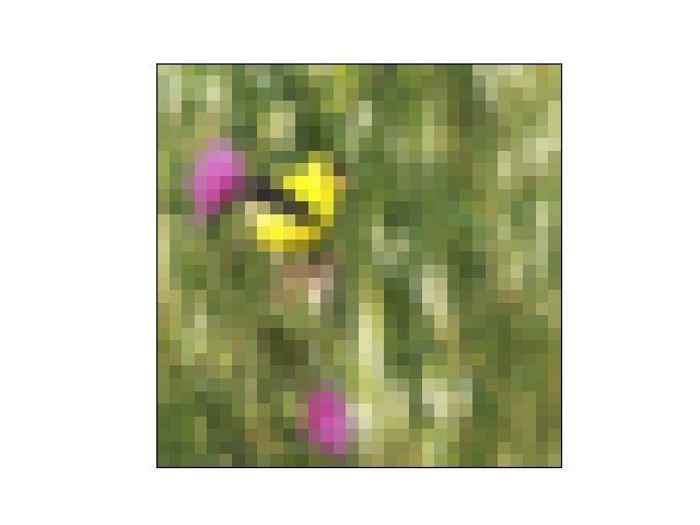
model. This corresponds to an objective such as (Eq. 1):             After each update of the labels, we normalize them so that
                                                                     they represent a valid probability distribution. This makes
    ỹ∗ = arg min` ((xt , yt ) , θ − α∇θ ` ((x̃, ỹ) , θ)) ,   (1)
              ỹ                                                     them interpretable and has led to improvements compared
                                                                     to unnormalized labels.
where ỹ are the distilled labels for base examples x̃, (xt , yt )
are the target set examples and labels and θ is the neural           Intuition. We analysed how the synthetic labels are meta-
network model learned with rate α and loss ` (we use cross-          learned by the second-order algorithm for a simple one-
entropy). We learn soft labels, so the dimensionality of each        layer model θ, with a sigmoid output unit and two classes
label is the number of classes C to distill. One gradient step       (details are in the supplementary).The meta-gradients     are:
                                                                     ∇ỹ L (fθ0 (x0t ) , yt0 ) = α σ θ0T x0t − yt0 x0T  0

is shown above, but in general there may be multiple steps.                                                         t x̃ .
    One option to achieve objective in (Eq. 1) would be to fol-      This shows that synthetic labels are updated proportionally
low Wang et al. (2018) and simulate the whole training pro-          to the similarity of the target dataset examples x0t and base
cedure for multiple gradient steps ∇θ within the inner loop.         examples x̃0 as well as the difference between the predic-
However, this requires back-propagating through a long in-           tions and true target set labels. Thus synthetic labels capture
ner loop, and ultimately requires a fixed training schedule          the different degrees of similarity between a base example
with optimized learning rates. We aim to produce a dataset           and examples from different classes in the target dataset. For
that can be used in a standard training pipeline downstream          example, in cross-dataset, the KMNIST ‘Ya’ has no cor-
(e.g. Adam optimizer with the default parameters).                   responding English symbol, but could be learned by partially
    Our first modification to the standard pipeline is to per-       assigning its label to similar looking English ‘X’s and ‘R’s.
form gradient descent iteratively on the model and the dis-          First-Order Version with Ridge Regression. To avoid
tilled labels, rather than performing many inner (model)             second-order gradients, we propose a first-order version that
steps for each outer (dataset) step. This increases efficiency       uses pseudo-gradient generated via a closed form solution
significantly due to a shorter compute graph for backprop-           to ridge regression. Ridge regression layers have previously
agation. Nevertheless, when there are very few training ex-          been used for few-shot learning (Bertinetto et al. 2019)
amples, the model converges quickly to an over-fitted local          within minibatch. However, we extend it to learn global
minimum, likely within a few hundred iterations. To man-             weights that persist across minibatches. Ridge regression
age this, our innovation is to detect overfitting when it oc-        can be defined and solved as:
curs, reset the model to a new random initialization and keep
                                                                                Wl = arg minkXW − Y k2 + λkW k2
training. Specifically, we measure the moving average of tar-                             W
get problem accuracy, and when it has not improved for set                                         −1 T                       (2)
number of iterations, we reset the model. This periodic reset                       = X T X + λI        X Y,
of the model after varying number of iterations is helpful for       where X are the image features, Y are the labels, W are the
learning labels that are useful for all stages of training and       ridge regression weights and λ is the regularization param-
thus less sensitive to the number of iterations used. To ensure      eter. Following Bertinetto et al. (2019), we use Woodbury
scalability to any number of examples, we sample a mini-             formula (Petersen and Pedersen 2012):
batch of base examples and synthetic labels and use those                                                   −1
to update the model, which also better aligns with standard                         Wl = X T XX T + λI          Y,             (3)
training practice. Once label distillation is done, we train a       which allows us to use matrix XX T with dimensionality
new model from scratch using random initial weights, given           depending on the square of the number of inputs (minibatch
the base examples and learned synthetic labels.                      size) rather than the square of the input embedding size. The
    We propose and evaluate two label distillation algorithms:       embedding size is typically significantly larger than the size
a second-order version that performs one update step within          of the minibatch, so it would make matrix inversion costly.
the inner loop; and a first-order version that uses a closed         While ridge regression (RR) is obviously oriented at regres-
form solution of ridge regression to find optimal classifier         sion problems, it has been shown (Bertinetto et al. 2019) to
weights for the base examples.                                       work well for classification when regressing label vectors.
Vanilla Second-Order Version. The training procedure                 Ridge Regression with Pseudo-Gradients. We use a RR
includes both inner and outer loop. The inner loop consists          layer as the final output layer of our base network – we
of one update of the model θ0 = θ − α∇θ L (fθ (x̃0 ) , ỹ0 ),        decompose the original model θ used for the second-order
through which we then backpropagate to update the syn-               version into feature extractor θ and RR classifier w. RR
thetic labels ỹ ← ỹ − β∇ỹ L (fθ0 (x0t ) , yt0 ). We perform       solves for the optimal (local) weights wl that classify the
a standard update of the model after updating the synthetic          features of the current minibatch examples. We exploit this
labels, which is more of a technical detail about how it is          local minibatch solution by taking a pseudo-gradient step
implemented rather than needed in theory as it could be              that updates global weights w as w ← (1 − α)w + αwl ,
combined with the inner-loop update. The method is oth-              with α being the pseudo-gradient step size. We can under-
erwise similar to our first-order ridge regression method,           stand this as a pseudo-gradient as it corresponds to the step
which is summarized in Algorithm 1, together with our no-            w ← w−α(w−wl ). We can then update the synthetic labels
tation. Note that examples from the target dataset are used          by back-propagating through local weights wl . Subsequent
when updating the synthetic labels ỹ, but for updating the          feature extractor updates on θ avoid second-order gradients.
model θ we only use synthetic labels and the base examples.          The full process is summarised in Algorithm 1.
Algorithm 1 Label distillation with ridge regression (RR)
 1: Input: x̃: N unlabeled examples from the base dataset; (xt , yt ): labeled examples from the target dataset; β: step size; α:
      pseudo-gradient step size; no , ni : outer (resp. inner) loop batch size; C number of classes in the target dataset
 2:   Output: distilled labels ỹ and a reasonable number of training steps Ti
 3:   ỹ ← 1/C                                                                                  //Uniformly initialize synthetic labels
 4:   θ ∼ p(θ)                                                                    //Randomly initialize feature extractor parameters
 5:   w←0                                                                                    // Initialize global RR classifier weights
 6:   while ỹ not converged do
 7:      (x̃0 , ỹ0 ) ∼ (x̃, ỹ)                                                          //Sample a minibatch of ni base examples
 8:      (x0t , yt0 ) ∼ (xt , yt )                                                      //Sample a minibatch of no target examples
 9:      wl = arg minL (fwl (fθ (x̃0 )) , ỹ0 )                                                                   // Solve RR problem
                  wl
10:   w ← (1 − α)w + αwl                                                                      //Update global RR classifier weights
11:   ỹ ← ỹ − β∇ỹ L (fw (fθ (x0t )) , yt0 )                                             //Update synthetic labels with target loss
12:   θ ← θ − β∇θ L (fw (fθ (x̃0 )) , ỹ0 )                                                              //Update feature extractor
13:   if L (fw (fθ (xt )) , yt ) did not improve then
14:      θ ∼ p(θ)                                                                                            //Reset feature extractor
15:      w←0                                                                                    // Reset global RR classifier weights
16:      Ti ← iterations since previous reset                                                                  //Record time to overfit
17:   end if
18: end while

                       4   Experiments                                  Sutskever, and Hinton 2012) for CIFAR-10, CIFAR-100 and
We perform two main types of experiments: (1) within-                   CUB. Both models are identical to the ones used in (Wang
dataset distillation, when the base examples come from the              et al. 2018). In a fully supervised setting they achieve about
target dataset and (2) cross-dataset distillation, when the             99% and 80% test accuracy on MNIST and CIFAR-10.
base examples come from a different but related dataset. The            Selection of Base Examples. The base examples are se-
dataset should be related because if there is a large shift in          lected randomly, using a shared random seed for consistency
the domain (e.g. from characters to photos), then the fea-              across scenarios. Our baseline models use the same random
ture extractor trained on the base examples would general-              seed as the distillation models, so they share base examples
ize poorly to the target dataset. We use MNIST, CIFAR-10                for fair comparison. For within-dataset label distillation, we
and CIFAR-100 for the task of within-dataset distillation,              create a balanced set of base examples, so each class has
while for cross-dataset distillation we use EMNIST (“En-                the same number of base examples. For cross-dataset label
glish letters”), KMNIST, Kuzushiji-49 (both “Japanese let-              distillation, we do not consider the original classes of base
ters”), MNIST (digits), CUB (birds) and CIFAR-10 (general               examples. The size of the label space and the labels are dif-
objects). Details of these datasets are in the supplementary.           ferent in the source and the target problem. Our additional
                                                                        analysis (Tables 6 and 7 in the supplementary) has shown
4.1     Experimental Settings                                           that the specific random set of base examples does not have
Monitoring Overfitting. We use parameters NM , NW to                    a significant impact on the success of label distillation.
say over how many iterations to calculate the moving aver-              Further Details. Outer loop minibatch size is no = 1024
age and how many iterations to wait before reset since the              examples, while the inner minibatch size ni depends on the
best moving average value. We select NM = NW and use a                  number of base examples used. When using 100 or more
value of 50 steps in most cases, while we use 100 for CIFAR-            base examples, we select a minibatch of 50 examples, except
100 and Kuzushiji-49, and 200 for other larger-scale experi-            for CIFAR-100 for which we use 100 examples. For 10, 20
ments (more than 100 base examples). These parameters do                and 50 base examples our minibatch sizes are 10, 10 and 25.
not affect the total number of iterations.                              We optimize the synthetic labels and the model itself using
Early Stopping for Learning Synthetic Labels. We up-                    Adam optimizer with the default parameters (β = 0.001).
date the synthetic labels for a given number of epochs and              Most of our models are trained for 400 epochs, while larger-
then select the best labels to use based on the validation per-         scale models (more than 100 base examples and CIFAR-
formance. For this, we train a new model from scratch using             100) are trained for 800 epochs. Smaller-scale Kuzushiji-
the current distilled labels and the associated base examples           49 experiments are trained for 100 epochs, while larger-
and then evaluate the model on the validation part of the tar-          scale ones use 200 epochs. Epochs are calculated based on
get set. We randomly set aside about 10-15% (depending on               the number of target set examples, rather than base exam-
the dataset) of the training data for validation.                       ples. In the second-order version, we perform one inner-
                                                                        loop step update, using a learning rate of α = 0.01. We
Models. We use LeNet (LeCun et al. 1998) for                            back-propagate through the inner-loop update when updat-
MNIST and similar experiments, and AlexNet (Krizhevsky,                 ing the synthetic labels (meta-knowledge), but not when
Base examples        10             20              50              100             200               500
                 LD               60.89 ± 3.20   74.37 ± 1.27    82.26 ± 0.88   87.27 ± 0.69     91.47 ± 0.53    93.30 ± 0.31
                 Baseline         48.35 ± 3.03   62.60 ± 3.33    75.07 ± 2.40   82.06 ± 1.75     85.95 ± 0.98    92.10 ± 0.43
      MNIST

                 Baseline LS      51.22 ± 3.18   64.14 ± 2.57    77.94 ± 1.26   85.95 ± 1.09     90.10 ± 0.60    94.75 ± 0.29
                 LD RR            64.57 ± 2.67   75.98 ± 1.00    82.49 ± 0.93   87.85 ± 0.43     88.88 ± 0.28    89.91 ± 0.33
                 Baseline RR      52.53 ± 2.61   60.44 ± 1.97    74.85 ± 2.37   81.40 ± 2.11     87.03 ± 0.69    92.10 ± 0.80
                 Baseline RR LS   51.53 ± 2.42   60.91 ± 1.78    76.26 ± 1.80   83.13 ± 1.41     87.94 ± 0.67    93.48 ± 0.61
                 DD                                                             79.5 ± 8.1
                 SLDD                                                           82.7 ± 2.8
                 LD               25.69 ± 0.72   30.00 ± 0.86    35.36 ± 0.64   38.33 ± 0.44     41.05 ± 0.71    42.45 ± 0.40
                 Baseline         14.29 ± 1.40   16.80 ± 0.72    20.75 ± 1.05   25.76 ± 1.04     31.53 ± 1.02    38.33 ± 0.75
      CIFAR-10

                 Baseline LS      13.22 ± 1.22   18.36 ± 0.65    22.81 ± 0.71   27.27 ± 0.68     33.62 ± 0.81    39.22 ± 1.12
                 LD RR            25.07 ± 0.69   29.83 ± 0.46    35.23 ± 0.64   37.94 ± 1.22     41.17 ± 0.33    43.16 ± 0.47
                 Baseline RR      13.37 ± 0.79   17.08 ± 0.31    19.85 ± 0.51   24.65 ± 0.47     28.97 ± 0.74    36.31 ± 0.49
                 Baseline RR LS   13.82 ± 0.85   16.95 ± 0.52    20.00 ± 0.57   24.84 ± 0.60     29.28 ± 0.56    35.73 ± 1.02
                 DD                                                             36.8 ± 1.2
                 SLDD                                                           39.8 ± 0.8

Table 1: Within-dataset distillation recognition accuracy (%). Our label distillation (LD) outperforms prior Dataset Distillation
(Wang et al. 2018) (DD) and SLDD (Sucholutsky and Schonlau 2019), and scales to synthesizing more examples.

subsequently updating the model θ with Adam optimizer.                However, this strategy has not shown to be effective enough
In the first-order version, we use a pseudo-gradient step size        for CIFAR-10, where synthetic labels are the best. Impor-
of 0.01 and λ of 1.0. We calibrate the regression weights             tantly, in the most intensively distilled regime of 10 exam-
by scaling them with a value learned during training with             ples, LD clearly outperforms all competitors. We provide an
the specific set of base examples and distilled labels. Our           analysis of the labels learned by our method in Section 4.5.
tables report the mean test accuracy and standard deviation           For CIFAR-10 our results also improve on the original DD
(%) across 20 models trained from scratch using the base              result. In this experiment, our second-order algorithm per-
examples and synthetic labels.                                        forms similarly to our RR pseudo-gradient strategy.

4.2         Within-Dataset Distillation
                                                                                    LD                  11.46 ± 0.39
We compare our label distillation (LD) to previous dataset                          Baseline             3.51 ± 0.31
distillation (DD) and soft-label dataset distillation (SLDD)                        Baseline LS          4.07 ± 0.23
on MNIST and CIFAR-10. We also establish new baselines                              LD RR               10.80 ± 2.36
that take true labels from the target dataset and otherwise                         Baseline RR          3.00 ± 0.39
are trained in the same way as LD models. RR baselines use                          Baseline RR LS       3.65 ± 0.28
RR and pseudo-gradient for consistency with LD RR (over-
all network architecture remains the same as in the second-
                                                                      Table 2: CIFAR-100 within-dataset distillation recognition
order approach). In addition, we include baselines that use
                                                                      accuracy (%). One example per class.
label smoothing (LS) (Szegedy et al. 2016) with a smooth-
ing parameter of 0.1 as suggested in (Pereyra et al. 2017).
The number of training steps for our baselines is optimized              We further show in Table 2 that our distillation approach
using the validation set, by training a model for various num-        scales to a significantly larger number of classes than 10 by
bers of steps between 10 and 1000 and measuring the vali-             application to the CIFAR-100 benchmark. As before, we es-
dation set accuracy (up to 1700 steps are used for cases with         tablish new baseline results that use the original labels (or
more than 100 base examples). The results in Table 1 show             their smoother alternatives) of the same images as those used
that LD significantly outperforms previous work on MNIST.             as base examples in distillation. We use the validation set to
This is in part due to LD enabling the use of more steps (LD          choose a suitable number of steps for training a baseline, al-
estimates Ti ≈ 200 − 300 steps vs fixed 3 epochs of 10 steps          lowing up to 1000 steps, which is significantly more than
in LD and SLDD). Our improved baselines are also com-                 what is typically used by LD. The results show our distilla-
petitive, and outperform the prior baselines in Wang et al.           tion method leads to clear improvements over the baseline.
(2018) due to taking more steps. However, since Wang et al.
(2018); Sucholutsky and Schonlau (2019) do not scale to               4.3   Cross-Dataset Task
more steps, this is a reasonable comparison. The standard             For cross-dataset distillation, we considered four scenarios:
uniform label smoothing baseline works well on MNIST for              from EMNIST letters to MNIST digits, from EMNIST let-
a large number of base examples, where the problem any-               ters (“English”) to Kuzushiji-MNIST or Kuzushiji-49 char-
way approaches one of conventional supervised learning.               acters (“Japanese”) and from CUB bird species to CIFAR-10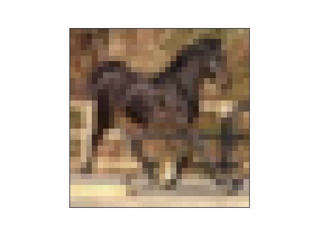
Base examples 10 20 50 100 200 500
E → M (LD) 36.13 ± 5.51 57.82 ± 1.91 69.21 ± 1.82 77.09 ± 1.66 83.67 ± 1.43 86.02 ± 1.00
E → M (LD RR) 56.08 ± 2.88 67.62 ± 3.03 80.80 ± 1.44 82.70 ± 1.33 84.44 ± 1.18 86.79 ± 0.76
E → K (LD) 31.90 ± 2.82 39.88 ± 1.98 47.93 ± 1.38 51.91 ± 0.85 57.46 ± 1.37 59.84 ± 0.80
E → K (LD RR) 34.35 ± 3.37 46.67 ± 1.66 53.13 ± 1.88 57.02 ± 1.24 58.01 ± 1.28 63.77 ± 0.71
B → C (LD) 26.86 ± 0.97 28.63 ± 0.86 31.21 ± 0.74 34.02 ± 0.66 38.39 ± 0.56 38.12 ± 0.41
B → C (LD RR) 26.50 ± 0.54 28.95 ± 0.47 32.23 ± 3.59 32.19 ± 7.89 36.55 ± 6.32 38.46 ± 6.97
E → K-49 (LD) 7.37 ± 1.01 9.79 ± 1.23 17.80 ± 0.78 19.17 ± 1.27 22.78 ± 0.98 23.99 ± 0.81
E → K-49 (LD RR) 10.48 ± 1.26 14.84 ± 1.83 21.59 ± 1.87 20.86 ± 1.81 24.59 ± 2.26 24.72 ± 1.78
Table 3: Cross-dataset distillation recognition accuracy (%). Datasets: E = EMNIST, M = MNIST, K = KMNIST, B = CUB, C
= CIFAR-10, K-49 = Kuzushiji-49.
20% fewer Original 20% more Original General optimizer AlexNet LeNet
100 86.67 86.98 Shuffled examples 50
CIFAR-10 test accuracy (%)
MNIST test accuracy (%)
100 38.39
MNIST test accuracy (%)
40 35.2
75 32.65
52.54 53.89 75
25.92
30
50
86.77 50
77.32 20
25 25 10
0 0 0
LD DD LD DD LD DD
(a) Optimization steps (b) Optimization parameters (c) Cross-architecture transfer
Figure 2: LD distilled datasets are more agnostic to optimization steps, hyperparameters, and network architecture than DD.
general categories. The results in Table 3 show we are able eters between meta-training + meta-testing. (3) How well the
to distill labels on examples of a different source dataset distilled datasets transfer to neural architectures different to
and achieve surprisingly good performance on the target those used for training. We used the DD implementation of
problem, given that no target data is used when training Wang et al. (2018) for fair evaluation. Figure 2 summarizes
these models. In contrast, directly applying a trained source- the key points, and detailed tables are in the supplementary.
task model to the target without distillation unsurprisingly
Sensitivity to the Number of Meta-Testing Steps (Fig-
leads to chance performance (about 2% test accuracy for
ure 2a). A key feature of our method is that it is relatively
Kuzushiji-49 and 10% for all other cases). These results
insensitive to the number of steps used to train a model on
show we can indeed distill the knowledge of one dataset into
the distilled data. Our results from Table 9 show that even
base examples from a different but related dataset through
if we do 50 steps less or 100 steps more than the number
crafting synthetic labels. Furthermore, our RR approach sur-
estimated during training (≈ 300), the testing performance
passes the second-order method in most cases, confirming its
does not change significantly. This is in contrast with previ-
value. When using 10 and 20 base examples for Kuzushiji-
ous DD and SLDD methods that must be trained for a spe-
49, the number of training examples is smaller than the
cific number of steps with optimized learning rates, making
number of classes (49), providing a novel example of less-
them rather inflexible. If the number of steps changes even
than-one-shot learning where there are fewer examples than
by as little as 20%, they incur a significant cost in accuracy.
classes (Sucholutsky and Schonlau 2020).
Table 10 provides a further analysis of sensitivity of DD.
4.4 Flexibility of Distilled Datasets Sensitivity to Optimization Parameters (Figure 2b). DD
We conduct experiments to verify the flexibility and gen- uses step-wise meta-optimized learning rates to maximize
eral applicability of our label-distilled dataset compared to accuracy. Our analysis in Table 11 shows that if we use an
image-distilled alternative by Wang et al. (2018). Namely, average of the optimized learning rate rather than the spe-
we looked at (1) How the number of steps used during meta- cific value in each step (more general optimizer), the perfor-
testing affects the performance of learning with the distilled mance decreases significantly. Further, original DD relies on
data, and in particular sensitivity to deviation from the num- training the distilled data in a fixed sequence, and our analy-
ber of steps used during meta-training of DD and LD. (2) sis in Table 12 shows changing the order of examples leads
Sensitivity of the models to changes in optimization param- to a large decrease in accuracy. Our LD method by design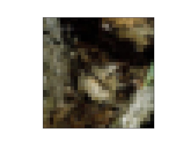
does not depend on the specific order of examples, and it                                                                 Second-order
can be used with off-the-shelf learning optimizers such as                                                                Pseudo-gradient RR
Adam to train the model, rather than with optimizers with                                            −10

                                                                                log(Var(gradient))
                                                                                                     −12
learning rates specific to the example and step.
                                                                                                     −14

Transferability of Labels Across Architectures (Fig-                                                 −16
                                                                                                     −18
ure 2c). We study the impact of distilling the labels using
                                                                                                     −20
AlexNet and then training AlexNet, LeNet and ResNet-18                                               −22
using the distilled labels. We establish new baselines for                                           −24
the additional architectures, using a number of steps chosen                                               0       200      400   600      800   1000
based on the validation set. Results in Tables 13 and 14 sug-                                                            Number of steps
gest our labels are helpful in both within and across dataset
distillation scenarios. This suggests that even if we relabel a    Figure 3: RR-based LD reduces synthetic label meta-
dataset with one label space to solve a different problem, the     gradient variance Var [∇ỹ L].
labels generalize to a new architecture and lead to improve-
ments over the baselines. We have done experiments with
original DD to find how robust it is to the change of archi-       on average, suggesting RR leads to more complex labels
tecture (Table 15). As expected, there is a large decrease in      that may better capture the different amounts of similar-
accuracy, but the results are better than the baselines they re-   ity of base examples to examples from different classes in
port (Wang et al. 2018), so their synthetic images are some-       the target dataset. This is also supported by visually simi-
what transferable when we train the model with the specific        lar digits such as 4 and 9 receiving more weight compared
order of examples and optimized learning rates. However,           to other combinations. For CIFAR-10, the labels are signifi-
our LD method incurs a smaller decrease in accuracy, sug-          cantly more complex, indicating non-trivial information is
gesting better transferability across architectures.               embedded into the synthetic labels. For cross-dataset LD
                                                                   (EMNIST base examples with KMNIST and MNIST target
4.5   Further Analysis                                             respectively), Figure 10 suggests LD can be understood as
Training Time. In Table 4 we compare training times of             learning labels such that the base examples’ label-weighted
our framework and the original DD (using the same set-             combination resembles the images from the target class. Ex-
tings and hardware). Besides evaluating LD, we also use our        amples of synthetic labels for both within and cross-dataset
meta-learning algorithm to implement an image-distillation         LD are also included in the supplementary.
strategy for direct comparison with the original DD. The           Pseudo-Gradient Analysis. To understand the superior
results show our online approach significantly accelerates         performance of our RR method, we analysed the variances
training. Our DD is comparable to LD, and both are faster          of meta-gradients obtained by our second-order and pseudo-
than original DD. However, we focus on LD because our              gradient methods. Results in Figure 3 show our pseudo-
version of DD was relatively unstable and led to worse per-        gradient RR method obtains a significantly lower variance
formance than LD, perhaps because learning synthetic im-           of meta-knowledge gradients, leading to more stable and ef-
ages is more complex than synthetic labels. This shows we          fective training.
need both the labels and our re-initializing strategy.
                                                                   Discussion. LD provides a more effective and more flexi-
                             MNIST       CIFAR-10                  ble distillation approach than prior work. This brings us one
                                                                   step closer to the vision of leveraging distilled data to accel-
           DD                  116          205                    erate model training, or design – such as architecture search
           LD                  61            86                    (Elsken, Metzen, and Hutter 2019). Currently we only ex-
           LD (RR)             65            98                    plicitly randomize over network initializations during train-
           Our DD              67            96                    ing. In future work we believe our strategy of multi-step
           Our DD (RR)         72            90                    training and reset at convergence could be used with other
                                                                   factors, such as randomly selected network architectures to
Table 4: Comparison of training times of DD (Wang et al.           further improve cross-network generalisation performance.
2018) and our LD (minutes).
                                                                                                               5         Conclusion
Analysis of Synthetic Labels. We have analysed to what             We have introduced a new label distillation algorithm for
extent the synthetic labels learn the true label and how this      distilling the knowledge of a large dataset into synthetic la-
differs between our second-order and RR methods (Figures           bels of a few base examples from the same or a different
8 and 9 in the supplementary). The results for a MNIST             dataset. Our method improves on prior dataset distillation
experiment with 100 base examples show the second-order            results, scales better to larger problems, and enables novel
method recovers the true value to about 84% on average,            settings such as cross-dataset distillation. Most importantly,
so it could be viewed as non-uniform label smoothing with          it is significantly more flexible in terms of distilling general
meta-learned weights on labels specific to the examples. For       purpose datasets that can be used downstream with off-the-
the same scenario, RR recovers the true value to about 63%         shelf optimizers.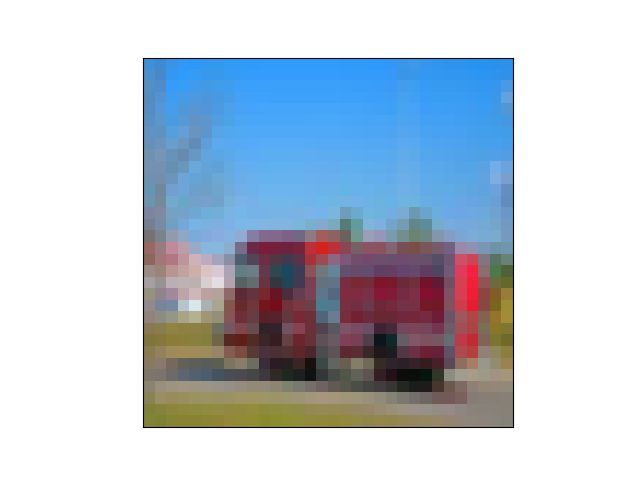
Ethics Statement                                Carlini, N.; Liu, C.; Erlingsson, U.; Kos, J.; and Song, D.
                                                                    2019. The secret sharer: evaluating and testing unintended
We propose a flexible and efficient distillation scheme that
                                                                    memorization in neural networks. In USENIX Security Sym-
gets us closer to the goal of practically useful dataset distil-
                                                                    posium.
lation. Dataset distillation could ultimately lead to a benefi-
cial impact in terms of researcher’s time efficiency by en-         Clanuwat, T.; Kitamoto, A.; Lamb, A.; Yamamoto, K.; and
abling faster experimentation when training on small dis-           Ha, D. 2018. Deep learning for classical Japanese literature.
tilled datasets. Perhaps more importantly, it could reduce the      In NeurIPS Workshop on Machine Learning for Creativity
environmental impact of AI research and development by re-          and Design.
duction of energy costs (Schwartz et al. 2019). However, our        Cohen, G.; Afshar, S.; Tapson, J.; and van Schaik, A. 2017.
results are still not strong enough yet. For this goal to be re-    EMNIST: an extension of MNIST to handwritten letters. In
alised better distillation methods leading to more accurate         arXiv.
downstream models need to be developed.
                                                                    Elsken, T.; Metzen, J. H.; and Hutter, F. 2019. Neural ar-
    In the future, label distillation could speculatively provide   chitecture search: a survey. Journal of Machine Learning
a useful tool for privacy preserving learning (Al-Rubaie and        Research 20: 1–21.
Chang 2019), for example in situations where organizations
want to learn from user’s data. A company could provide             Farquhar, G.; Whiteson, S.; and Foerster, J. 2019. Loaded
a small set of public (source) data to a user, who performs         DiCE: Trading off Bias and Variance in Any-Order Score
cross-dataset distillation using their private (target) data to     Function Estimators for Reinforcement Learning.            In
train a model. The user would then return the distilled labels      NeurIPS.
on the public data, which would allow the company to re-            Felzenszwalb, P. F.; Girshick, R. B.; McAllester, D.; and
create the user’s model. In this way the knowledge from the         Ramanan, D. 2010. Object detection with discriminatively
user’s training could be obtained by the company in the form        trained part-based models. IEEE Transactions on Pattern
of distilled labels – without directly sending any private data,    Analysis and Machine Intelligence 32(9): 1627–1645.
or trained model that could be a vector for memorization            Finn, C.; Abbeel, P.; and Levine, S. 2017. Model-agnostic
attacks (Carlini et al. 2019).                                      meta-learning for fast adaptation of deep networks. In
    On the negative side, detecting and understanding the im-       ICML.
pact of bias in datasets is an important yet already very chal-
lenging issue for machine learning. The impact of dataset           Hinton, G.; Vinyals, O.; and Dean, J. 2014. Distilling the
distillation on any underlying biases in the data is com-           knowledge in a neural network. In NIPS.
pletely unclear. If people were to train models on distilled        Hospedales, T.; Antoniou, A.; Micaelli, P.; and Storkey, A.
datasets in the future, it would be important to understand         2020. Meta-learning in neural networks: a survey. In arXiv.
the impact of distillation on data biases.                          Krizhevsky, A. 2009. Learning multiple layers of features
                                                                    from tiny images. Technical report.
                       Source Code                                  Krizhevsky, A.; Sutskever, I.; and Hinton, G. E. 2012. Im-
We provide a PyTorch implementation of our approach at              ageNet classification with deep convolutional neural net-
https://github.com/ondrejbohdal/label-distillation.                 works. In NIPS.
                                                                    LeCun, Y.; Bottou, L.; Bengio, Y.; and Haffner, P. 1998.
                   Acknowledgments                                  Gradient-based learning applied to document recognition.
                                                                    Proceedings of the IEEE 86(11): 2278–2324.
This work was supported in part by the EPSRC Centre for
Doctoral Training in Data Science, funded by the UK En-             Lee, K.; Maji, S.; Ravichandran, A.; and Soatto, S. 2019.
gineering and Physical Sciences Research Council (grant             Meta-learning with differentiable convex optimization. In
EP/L016427/1) and the University of Edinburgh.                      CVPR.
                                                                    Li, Y.; Yang, Y.; Zhou, W.; and Hospedales, T. M. 2019.
                        References                                  Feature-critic networks for heterogeneous domain general-
                                                                    ization. In ICML.
Al-Rubaie, M.; and Chang, J. M. 2019. Privacy-preserving
                                                                    Liu, H.; Socher, R.; and Xiong, C. 2019. Taming MAML:
machine learning: threats and solutions. IEEE Security and
                                                                    Efficient Unbiased Meta-Reinforcement Learning. In ICML.
Privacy 17(2): 49–58.
                                                                    Lorraine, J.; Vicol, P.; and Duvenaud, D. 2020. Optimizing
Angelova, A.; Abu-Mostafa, Y.; and Perona, P. 2005. Prun-           Millions of Hyperparameters by Implicit Differentiation. In
ing training sets for learning of object categories. In CVPR.       AISTATS.
Balaji, Y.; Sankaranarayanan, S.; and Chellappa, R. 2018.           Luketina, J.; Berglund, M.; Klaus Greff, A.; and Raiko, T.
MetaReg: towards domain generalization using meta-                  2016. Scalable Gradient-Based Tuning of Continuous Reg-
regularization. In NeurIPS.                                         ularization Hyperparameters. In ICML.
Bertinetto, L.; Henriques, J.; Torr, P. H. S.; and Vedaldi,         Maclaurin, D.; Duvenaud, D.; and Adams, R. P. 2015.
A. 2019. Meta-learning with differentiable closed-form              Gradient-based Hyperparameter Optimization through Re-
solvers. In ICLR.                                                   versible Learning. In ICML.
Micaelli, P.; and Storkey, A. 2019. Zero-shot knowledge
transfer via adversarial belief matching. In NeurIPS.
Nichol, A.; Achiam, J.; and Schulman, J. 2018. On first-
order meta-learning algorithms. In arXiv.
Olvera-López, J. A.; Carrasco-Ochoa, J. A.; Martı́nez-
Trinidad, J. F.; and Kittler, J. 2010. A review of instance se-
lection methods. Artificial Intelligence Review 34(2): 133–
143.
Pereyra, G.; Tucker, G.; Chorowski, J.; Kaiser, L.; and Hin-
ton, G. 2017. Regularizing neural networks by penalizing
confident output distributions. In arXiv.
Petersen, K. B.; and Pedersen, M. S. 2012. The matrix cook-
book. Technical report.
Schwartz, R.; Dodge, J.; Smith, N. A.; and Etzioni, O. 2019.
Green AI. In arXiv.
Sener, O.; and Savarese, S. 2018. Active learning for convo-
lutional neural networks: A core-set approach. In ICLR.
Shleifer, S.; and Prokop, E. 2019. Proxy Datasets for Train-
ing Convolutional Neural Networks. In arXiv.
Sucholutsky, I.; and Schonlau, M. 2019. Soft-label dataset
distillation and text dataset distillation. In arXiv.
Sucholutsky, I.; and Schonlau, M. 2020. ’Less Than One’-
Shot Learning: Learning N Classes From M
A Datasets after which we update the synthetic label:
ỹ ← ỹ − β∇ỹ L σ(θ0T xt ), yt .
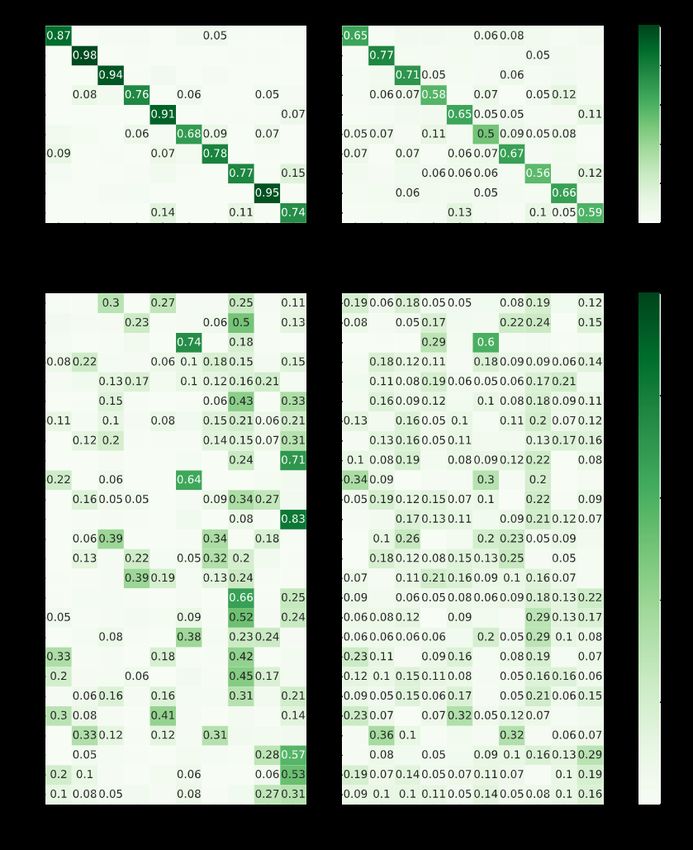
We use MNIST (LeCun et al. 1998), EMNIST (Cohen et al.
2017), KMNIST and Kuzushiji-49 (Clanuwat et al. 2018), Notation: x̃ is the base example, ỹ is the synthetic label, α
CIFAR-10 and CIFAR-100 (Krizhevsky 2009), and CUB is the inner-loop learning rate, β is the outer-loop learning
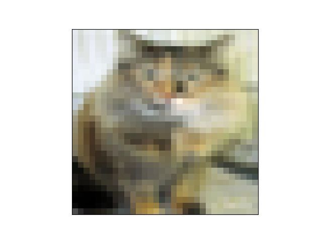
(Wah et al. 2011) datasets. Example images are shown in rate, xt is the target set example, yt is the label of the target
Figure 4. MNIST includes images of 70000 handwritten dig- set example and θ describes the model weights.
its that belong into 10 classes. EMNIST dataset includes Our goal is to intuitively interpret the update of the syn-
various characters, but we choose EMNIST letters split that thetic label, which uses the gradient ∇ỹ L σ(θ0T xt ), yt .
includes only letters. Lowercase and uppercase letters are We will repeatedly use the chain rule and the fact that
combined together into 26 balanced classes (145600 exam-
ples in total). KMNIST (Kuzushiji-MNIST) is a dataset that ∂σ(x)
= σ(x) (1 − σ(x)) .
includes images of 10 classes of cursive Japanese (Kuzushiji) ∂x
characters and is of the same size as MNIST. Kuzushiji-49 Moreover, we will use the following result (for binary cross-
is a larger version of KMNIST with 270912 examples and entropy loss L introduced earlier):
49 classes. CIFAR-10 includes 60000 colour images of vari- ∂L σ(θT x), y
∂L σ(θT x), y ∂σ(θT x)
ous general objects, for example airplanes, frogs or ships. As =
the name indicates, there are 10 classes. CIFAR-100 is like ∂θ ∂σ(θT x) ∂θ
T
CIFAR-100, but has 100 classes with 600 images for each of = y − σ(θ x) x
them. Every class belongs to one of 20 superclasses which
Now we derive an intuitive formula for the gradient used
represent more general concepts. CUB includes colour im-
for updating the synthetic label:
ages of 200 bird species. The number of images is relatively
∂L σ(θ0T xt ), yt
small, only 11788. All datasets except Kuzushiji-49 are bal- ∂L (ŷt0 , yt )
anced or almost balanced. =
∂ ỹ ∂ ỹ
T
∂L (ŷt0 , yt ) ∂ ŷt0 ∂θ0
= 0 0
MNIST
∂ ŷt ∂θ ∂ ỹ
0 T ∂ θ − α∇ L σ(θ T x̃), ỹ
0
∂L (ŷt , yt ) ∂ ŷt θ
=
EMNIST ∂ ŷt0 ∂θ0 ∂ ỹ
T
∂L (ŷt0 , yt ) ∂ ŷt0 ∂ θ − α ỹ − σ(θT x̃) x̃
=
Kuzushiji ∂ ŷt0 ∂θ0 ∂ ỹ
0 0 T
∂L (ŷt , yt ) ∂ ŷt
= (−αx̃)
CIFAR-10
∂ ŷt0 ∂θ0
T
= ((yt − ŷt0 ) xt ) (−αx̃)
= α σ(θ0T xt ) − yt xTt x̃
CUB
The next step is to interpret the update rule. The update
is proportional to the difference between the prediction on
the target set and the true label σ(θ0T xt ) − yt as well as
Figure 4: Example images from the different datasets that
we use. to the similarity between the target set example and the base
example xTt x̃ . This suggests the synthetic labels are up-
dated so that they capture the different amount of similarity
of a base example to examples from different classes in the
target dataset. A similar analysis can also be done for our RR
B Analysis of Simple One-Layer Case method – in such case the result would be similar and would
In this section we analyse how synthetic labels are meta- include a further proportionality constant dependent on the
learned in the case of a simple one-layer model with sig- base examples (not affecting the intuitive interpretation).
moid output layer σ, second-order approach and binary clas-
sification problem. We will consider one example at a time C Additional Experimental Details
for simplicity. The model has weights θ and gives predic- Normalization. We normalize greyscale images using the
tion ŷ = σ(θT x) for input image x with true label y. standardly used normalization for MNIST (mean of 0.1307
We use binary cross-entropy loss: L (ŷ, y) = y log ŷ + and standard deviation of 0.3081). All our greyscale images
(1 − y) log (1 − ŷ) . are of size 28 × 28. Colour images are normalized using
As part of the algorithm, we first update the base model, CIFAR-10 normalization (means of about 0.4914, 0.4822,
using the current base example and synthetic label: 0.4465, and standard deviations of about 0.247, 0.243, 0.261
across channels). All colour images are reshaped to be of
θ0 = θ − α∇θ L σ(θT x̃), ỹ ,
size 32 × 32.Computational Resources. Each experiment was done on larger. In fact, future work could investigate how to choose
a single GPU, in almost all cases NVIDIA 2080 Ti. Shorter base examples so that learning synthetic labels for them im-
(400 epochs) experiments took about 1 or 2 hours to run, proves the result further. We have tried the following strat-
while longer (800 epochs) experiments took between 2 and egy, but the label distillation results remained similar to the
4 hours. previous results (the new results are in Table 7):
In addition, Figure 5 illustrates the difference between a • Try 50 randomly selected sets of examples, train a model
standard model used for second-order label distillation and with each three times (for robustness) and measure the
a model that uses global ridge regression classifier weights validation accuracy.
(used for first-order RR label distillation). The two models
are almost identical – only the final linear layer is different. • The validation accuracy is measured for various numbers
of steps, in most cases we evaluate every 50 steps up to
1000 steps (with some additional small number of steps at
Standard Model with ridge the beginning). If there are more than 100 base examples,
model regression weights we allow up to 1700 steps.
Input Input
• Select the set with the largest mean validation accuracy at
any point of training (across the three runs).
• This strategy maximizes the performance of the baselines,
Feature extractor Feature extractor but could potentially also help the label distillation since
with CNN layers with CNN layers
these examples could be generally better for training.
Dependence on Target Dataset Size. Our experiments
Linear layer Linear layer use a relatively large target dataset (about 50000 exam-
ples) for meta-learning. We study the impact of reducing the
ReLU ReLU amount of target data for distillation in Table 8. Using 5000
non-linearity non-linearity or more examples (about 10% of the original size) is enough
to achieve comparable performance.
Linear layer Linear layer
Transferability of RR Synthetic Labels to Standard
ReLU ReLU Model Training. When using RR, we train a validation
non-linearity non-linearity and test model with RR and global classifier weights ob-
tained using pseudo-gradient. In this experiment we study
Global RR
Linear layer
classifier weights
what happens if we create synthetic labels with RR, but
do validation and testing with standard models trained from
scratch without RR. For a fair comparison, we use the same
Prediction Prediction
synthetic labels for training a new RR model and a new
standard model. Validation for early stopping is done with
a standardly trained model. The results in Table 16 suggest
Figure 5: Comparison of a standard model used for second- RR labels are largely transferable (even in cross-dataset sce-
order label distillation and a model that uses global ridge narios), but there is some decrease in performance. Conse-
regression classifier weights (used for first-order RR label quently, it is better to learn the synthetic labels using second-
distillation). order approach if we want to train a standard model without
RR during testing (comparing with the results in Table 1, 2
and 3).
Intuition on Cross-Dataset Distillation. To illustrate the
D Additional Experiments mechanism behind cross-dataset distillation, we use the dis-
Stability and Dependence on Choice of Base Examples. tilled labels to linearly combine base EMNIST example im-
To evaluate the consistency of our results, we repeat the en- ages weighted by their learned synthetic labels in order to es-
tire pipeline and report the results in Table 5. In the previous timate a prototypical KMNIST/MNIST target class example
experiments, we used one randomly chosen but fixed set of as implied by learned LD labels. Although the actual mech-
base examples per source task. We investigate the impact of anism is more complex than this due to the non-linearity of
base example choice by drawing further random base exam- the neural network, we can qualitatively see individual KM-
ple sets. The results in Table 6 suggest that the impact of NIST/MNIST target classes are approximately encoded by
base example choice is slightly larger than that of the vari- their linear EMNIST LD prototypes as shown in Figure 10.
ability due to the distillation process, but still small overall.
Note that the ± standard deviations in all cases quantify the E Results of Analysis
impact of retraining from different random initializations at Our tables report the mean test accuracy and standard de-
meta-test, given a fixed base set and completed distillation. viation (%) across 20 models trained from scratch using the
It is likely that if the base examples were not selected ran- base examples and synthetic labels. When analysing original
domly, the impact of using specific base examples would be DD, 200 randomly initialized models are used.Trial 1 Trial 2 Trial 3
MNIST (LD) 87.27 ± 0.69 87.49 ± 0.44 86.77 ± 0.77
MNIST (LD RR) 87.85 ± 0.43 88.31 ± 0.44 88.07 ± 0.46
E → M (LD) 77.09 ± 1.66 76.81 ± 1.47 77.10 ± 1.74
E → M (LD RR) 82.70 ± 1.33 83.06 ± 1.43 81.46 ± 1.70
Table 5: Repeatability. Label distillation is quite repeatable. Performance change from repeating the whole distillation learning
and subsequent re-training is small. We used 100 base examples for these experiments. Datasets: E = EMNIST, M = MNIST.
Set 1 Set 2 Set 3 Set 4 Set 5
MNIST (LD) 84.91 ± 0.92 87.38 ± 0.81 87.49 ± 0.44 87.12 ± 0.47 85.16 ± 0.48
MNIST (LD RR) 87.82 ± 0.60 88.78 ± 0.57 88.31 ± 0.44 88.40 ± 0.46 87.77 ± 0.60
E → M (LD) 79.34 ± 1.36 74.55 ± 1.00 76.81 ± 1.47 78.59 ± 1.05 78.55 ± 1.32
E → M (LD RR) 81.67 ± 1.39 83.30 ± 1.38 83.06 ± 1.43 82.62 ± 1.70 83.43 ± 0.98
Table 6: Base example sensitivity. Label distillation has some sensitivity to the specific set of base examples (chosen by a
specific random seed), but the sensitivity is relatively low. We used 100 base examples for these experiments. It is likely that
label distillation would be more sensitive for a smaller number of base examples.
Base examples 10 20 50 100 200 500
LD 66.96 ± 2.01 74.37 ± 1.65 83.17 ± 1.28 86.66 ± 0.44 90.75 ± 0.49 93.22 ± 0.41
Baseline 56.60 ± 3.10 64.77 ± 1.90 77.33 ± 2.51 84.86 ± 1.16 88.33 ± 1.04 92.87 ± 0.67
MNIST
Baseline LS 60.44 ± 2.05 66.41 ± 2.14 80.54 ± 1.94 86.98 ± 0.99 91.12 ± 0.79 95.56 ± 0.18
LD RR 71.34 ± 2.19 73.34 ± 1.18 84.66 ± 0.89 88.30 ± 0.46 88.91 ± 0.36 89.73 ± 0.39
Baseline RR 59.20 ± 2.18 65.22 ± 2.29 77.34 ± 1.68 84.70 ± 0.81 87.87 ± 0.68 92.39 ± 0.53
Baseline RR LS 60.63 ± 1.64 65.61 ± 1.08 77.39 ± 1.67 85.63 ± 0.95 88.89 ± 0.88 94.33 ± 0.44
DD 79.5 ± 8.1
SLDD 82.7 ± 2.8
LD 26.65 ± 0.94 29.07 ± 0.62 35.03 ± 0.48 38.17 ± 0.36 42.12 ± 0.56 41.90 ± 0.28
Baseline 17.57 ± 1.63 21.66 ± 0.91 23.59 ± 0.80 27.79 ± 1.01 33.49 ± 0.77 40.44 ± 1.33
CIFAR-10
Baseline LS 18.57 ± 0.68 22.91 ± 0.70 24.57 ± 0.83 29.27 ± 0.85 34.83 ± 0.75 40.15 ± 0.66
LD RR 25.08 ± 0.39 28.17 ± 0.34 34.43 ± 0.38 37.59 ± 1.68 42.48 ± 0.25 44.81 ± 0.26
Baseline RR 18.42 ± 0.59 21.00 ± 0.73 22.45 ± 0.49 24.46 ± 1.67 30.96 ± 0.49 39.17 ± 0.47
Baseline RR LS 18.22 ± 0.67 22.31 ± 1.01 22.27 ± 0.75 24.84 ± 2.89 30.74 ± 0.80 38.86 ± 0.88
DD 36.8 ± 1.2
SLDD 39.8 ± 0.8
Table 7: Optimized base examples: within-dataset distillation recognition accuracy (%). Our label distillation (LD) outperforms
prior Dataset Distillation (Wang et al. 2018) (DD) and SLDD (Sucholutsky and Schonlau 2019), and scales to synthesizing
more examples. The LD results remained similar to the original results even with optimized base examples.
Target examples 100 500 1000 5000 10000 20000 All
E → M (LD) 50.70 ± 2.33 61.92 ± 3.62 57.39 ± 4.58 75.44 ± 1.60 76.79 ± 1.12 77.27 ± 1.25 77.09 ± 1.66
E → M (LD RR) 60.67 ± 3.17 72.09 ± 2.40 65.71 ± 3.77 76.83 ± 2.33 80.66 ± 1.97 82.44 ± 1.64 82.70 ± 1.33
Table 8: Dependence on target set size. Around 5000 examples (≈ 10% of all data) is sufficient. Similarly as before, we used
100 base examples. Using all examples means using 50000 examples.You can also read