FES2014 global ocean tide atlas: design and performance
←
→
Page content transcription
If your browser does not render page correctly, please read the page content below
Ocean Sci., 17, 615–649, 2021
https://doi.org/10.5194/os-17-615-2021
© Author(s) 2021. This work is distributed under
the Creative Commons Attribution 4.0 License.

FES2014 global ocean tide atlas: design and performance
Florent H. Lyard1 , Damien J. Allain1 , Mathilde Cancet2 , Loren Carrère3 , and Nicolas Picot4
1 LEGOS, Université de Toulouse, CNES, CNRS, IRD, Toulouse, France
2 NOVELTIS, Labège, 31670, France
3 CLS, Ramonville-Saint-Agne, 31520, France
4 DSO/OT, CNES, Toulouse, 31400, France

Correspondence: Florent H. Lyard (florent.lyard@legos.obs-mip.fr)

Received: 6 October 2020 – Discussion started: 16 October 2020
Revised: 21 February 2021 – Accepted: 22 February 2021 – Published: 5 May 2021

Abstract. Since the mid-1990s, a series of FES (finite ele-       1   Introduction
ment solution) global ocean tidal atlases has been produced
and released with the primary objective to provide altimetry
missions with tidal de-aliasing correction at the best possible   The FES2014 global ocean atlas is the latest release of a 20-
accuracy. We describe the underlying hydrodynamic and data        year effort to improve tidal predictions needed in satellite al-
assimilation design and accuracy assessments for the latest       timetry de-aliasing. It is based on the hydrodynamic mod-
FES2014 release (finalized in early 2016), especially for the     elling of tides (Toulouse Unstructured Grid Ocean model,
altimetry de-aliasing purposes. The FES2014 atlas shows ex-       further denoted T-UGOm) coupled to an ensemble data as-
tremely significant improvements compared to the standard         similation code (spectral ensemble optimal interpolation, de-
FES2004 and (intermediary) FES2012 atlases, in all ocean          noted SpEnOI). It is a very significant upgrade compared to
compartments, especially in shelf and coastal seas, thanks        both the FES2004 (Lyard et al., 2006) and FES2012 (Stam-
to the unstructured grid flexible resolution, recent progress     mer et al., 2014) atlases, thanks to the improvement of the as-
in the (prior to assimilation) hydrodynamic tidal solutions,      similated data accuracy and the model performance. To some
and use of ensemble data assimilation technique. Compared         extent, FES2014 can be considered as an iterative step of
to earlier releases, the available tidal constituent’s spectrum   the FES2012 atlas, mostly motivated by the overwhelming
has been significantly extended, the overall resolution has       progress made in the hydrodynamic solutions accuracy to-
been augmented, and additional scientific byproducts such         ward the end of the FES2012 project and which could not be
as loading and self-attraction, energy diagnostics, or lowest     incorporated due to the project schedules. As will be further
astronomical tides have been derived from the atlas and are       mentioned in this publication, the efficiency of data assim-
available. Compared to the other available global ocean tidal     ilation increases significantly with prior solutions accuracy
atlases, FES2014 clearly shows improved de-aliasing per-          and for two main reasons. First, despite a rigorous theoret-
formance in most of the global ocean areas and has conse-         ical framework, data assimilation relies on strong assump-
quently been integrated in satellite altimetry geophysical data   tions in which the choice of the vector norm chosen to build
records (GDRs) and gravimetric data processing and adopted        the penalty function is critical (the most commonly used
in recently renewed ITRF standards (International Terres-         norm is the L2 norm, which is consistent with a Gaussian-
trial Reference System, 2020). It also provides very accurate     shaped error probability density assumption and which leads
open-boundary tidal conditions for regional and coastal mod-      to easily resolved linear systems but also which tends to
elling.                                                           over-weight outliers in data or simulation values; see Ben-
                                                                  nett, 1992, and Tarantola, 2005). Data assimilation must also
                                                                  be fed with quasi-empirical, partially subjective parameters,
                                                                  such as error covariances assigned to datasets. So while cor-
                                                                  recting prior (hydrodynamic) solution errors, it can also in-
                                                                  ject some methodological errors in the assimilation solutions,

Published by Copernicus Publications on behalf of the European Geosciences Union.
616                                                                       F. H. Lyard et al.: FES2014 global ocean tide atlas

more or less proportional to the prior distance between the      usual mass-conservative equilibrium approximation) to the
observations and the numerical solutions. Second, as we use      FES2014b atlas. It must be noticed that similar long-period
an ensemble technique to assess the prior modelling error        constituents are implicitly added in tidal prediction if no
covariances, and as those covariances will strongly dictate      corresponding external solution file is provided. To avoid
data assimilation innovation in model regions where assimi-      confusion in public releases, the extended FES2014b atlas
lation data density is very sparse (sparse must be understood    has received the FES2014c denomination.
as compared to the tidal wavelength, hence being quite differ-      The objectives of our communication are to concisely
ent in shallow-water seas compared to deep ocean regions),       present the FES2014 atlas main construction details, the val-
the prior hydrodynamic realism is critical to consistently       idation diagnostics, and the available byproducts, and not to
propagate information from data locations (where data/prior      propose a dissertation about tidal science findings based on
model trade-off is actually solved) toward “remote” model        this atlas which would lead us much too far. Consequently,
regions. Therefore, considering the significant potential im-    in the following sections, we intend to provide to the reader
provements, and thanks to the financial support of CNES          with information on the major ingredients of the FES2014
(Centre National d’Etudes Spatiales), the decision was made      atlas production (hydrodynamic modelling, data processing,
to rapidly upgrade the FES2012 atlas toward the FES2014          and data selection for assimilation and validation, assimila-
atlas.                                                           tion processing) and a basic accuracy assessment overview.
   The FES (finite element solution) atlas series started with   Complementary to the present publication, some additional
the FES94 release, quickly followed with the FES95 one           information on present and earlier FES atlases and a link
(Shum et al., 1997; Le Provost et al., 1997), which included     to the associated prediction software can be found on the
some upgrades and fixes for various issues detected after        Aviso+ website.
the FES94 official release. A similar scenario occurred for
the FES98 and FES99 (Lefevre et al., 2002), FES2002 and
FES2004, and FES2012 and FES2014 atlas production. De-           2     Hydrodynamic prior solutions
spite intensive quality checking during the production phase,
any new major version of FES atlas release is followed           One primary objective in the FES2014 atlas production is
by an extended verification/validation phase from the FES        to dynamically model the ocean tides with the best possi-
team and other worldwide specialists through the science         ble accuracy and to keep the data assimilation correction as
applications that use the new atlas. The upgrading/fixing        limited as feasible, hence limiting the atlas dependence upon
step is limited to issues that do not demand any major           altimetry-derived data and altimetry errors (Zawadzki et al.,
changes in the production process (such as unstructured grid     2018).
modifications) but still will bring valuable improvements
for the final user. The FES2014 atlas denomination is            2.1    T-UGOm time-stepping and frequency-domain
quite misleading, as its final version has been delivered               solvers
in early 2016. This has left time to the project team to
precisely assess the FES2014 accuracy and performance            T-UGOm (mercurial repository at https://hg.legos.obs-mip.
in altimetry data de-aliasing correction and to make some        fr/tugo/, last access: 28 March 2021) is a 2-D / 3-D unstruc-
final adjustments to guarantee the best possible quality at      tured grid model developed at the Laboratoire d’Etudes en
that time. It results in three available FES2014 releases.       Géophysique et Océanographie Spatiales (LEGOS). It can
FES2014a is the first guess based on a data assimilation         accommodate a variety of numerical discretizations (con-
set where altimetry data were corrected from tidal loading       tinuous and discontinuous finite elements, finite volumes)
provided by the GOTv8 model (Desai and Ray, 2014). Its           on triangle or quadrangle elements, based on the usual
production allowed for internal verification checks and data     Navier–Stokes equation in the Boussinesq approximation,
assimilation adjustments and finally the production of the       with a non-hydrostatic pressure solver available. It can be
self-consistent FES2014a tidal loading atlas used within         used in time-stepping (TS) or frequency-domain (FD) mode.
the FES2014b altimetry assimilation data processing. The         In 2005, based on FES2004 experience, an internal tide
FES2014a atlas was not intended to be widely distributed         wave drag parameterization (ITWD) has been implemented
or advertised. FES2014b was the first official release and,      for 2-D shallow-water simulations (characterizing the en-
after regridding from the native unstructured grid onto a        ergy transfer from the barotropic tides to the internal, baro-
regular 1/16◦ resolution grid, it has been made available        clinic tides). The ITWD parameterization, originally devel-
on the Aviso+ website (https://www.aviso.altimetry.fr/en/        oped from the pioneering work of Bell (1975) and Baines
data/products/auxiliary-products/global-tide-fes.html, last      (1982), proved to be essential in tidal and storm surges sim-
access: 28 March 2021). To provide a more comprehensive,         ulation accuracy, as tidal energy conversion accounts for
coherent tidal spectrum for tidal predictions particularly       a significant portion of the total barotropic energy dissipa-
for the geodetic community, several long-period tide con-        tion. Most of the critical dynamical parameters (such as bot-
stituents were explicitly added in 2019 (computed from the       tom roughness, internal tide drag coefficient, etc.) can be

Ocean Sci., 17, 615–649, 2021                                                         https://doi.org/10.5194/os-17-615-2021
F. H. Lyard et al.: FES2014 global ocean tide atlas                                                                            617

non-uniformly prescribed inside the domain. Initially, the         we will confine ourselves to the main differences between
frequency-domain mode has been integrated in the origi-            the CEFMO and T-UGOm formulations. The FES2014 mesh
nal T-UGOm time-stepping code to dynamically and con-              is built on triangle elements. Various numerical discretiza-
sistently downscale tidal boundary conditions for domain-          tions for elevations and currents can be defined on triangle
limited, time-stepping simulations (actually, some classes         elements, i.e. continuous or discontinuous, high or low or-
of open-boundary-condition time-stepping schemes, such as          der. Since its early releases, the FES tidal atlas mesh has
Riemann invariants, require prescribing tidal velocities in        been designed in terms of spatial resolution for continuous
conjunction with tidal elevations. Contrary to elevations, ve-     LGP2 discretization (quadratic Lagrange polynomial basis
locities are very sensitive to bathymetry and grid resolution,     functions, allowing for about 4 times more numerical nodes
and a simple interpolation from a global atlas, with different     compared to linear Lagrange polynomials, denoted LGP1).
bathymetry and resolution, may not meet the necessary con-         Among other available options, tidal velocity discretization
sistency with the domain-limited configuration. A FD simu-         is an element-wise discontinuous non-conforming linear in-
lation, where only elevations are prescribed at open bound-        terpolation function (NCP1). This choice has two major ad-
aries, will produce a properly downscaled velocity field over      vantages: the elevation gradient discrete space is identical to
the domain-limited grid, including open boundaries). The FD        the tidal current space, and the discrete momentum equation
solver is run for each tidal component separately. It basi-        system is diagonal, easing the construction and solving of the
cally assembles a frequency-domain wave equation and the           wave equation. Non-diagonal terms, such as horizontal mo-
solution is obtained by a simple inversion of the system.          mentum diffusion, must be left in the right-hand side vector
Naturally, the FD solver is based upon linearized equations,       and converged in an iterative manner or simply dismissed
and subsequently non-linear processes require an iterative         (in time-stepping codes, momentum diffusion acts mostly
approach to converge toward the fully non-linear solutions.        as a temporal scheme stabilizer, which is not needed in the
The number of iterations is rather limited for the major as-       frequency-domain solver). Tidal currents are expressed un-
tronomical tidal components; it tends to increase when ad-         der a standard Galerkin procedure, and this is one of the ma-
dressing compound tides and overtides. In any case, the nu-        jor differences with the CEFMO model where currents were
merical cost of the FD solver is extremely small compared to       estimated at numerical integration nodes (Gauss quadrature).
the TS solver cost (more than 1000 times smaller). In terms
of solution accuracy, FD and TS solvers are quite equiva-          2.3   TS discrete equations
lent, with of course a limited advantage to the TS solver in
non-linear tide cases. Therefore, in the perspective of data       Quite similarly to the FD equation, the TS 2-D shallow-
assimilation using ensembles for the major ocean tides com-        water equations in T-UGOm are based on the so-called gen-
ponents, the ensemble members have been computed in the            eralized wave equation. Inspired by Lynch and Gray (1979),
FD mode (details of data assimilation are described in a ded-      and continuously developed since, the approach has evolved
icated section of the article). Another major advantage of the     from application to the global ocean, now up to the inclu-
FD solver’s reduced numerical cost is the possibility to con-      sion of nearshore and estuarine numerical applications, with
duct a wide range of experiments in order to (globally or re-      wetting–drying and non-hydrostatic (surface wave dynam-
gionally) test numerical developments, calibrate the model         ics) capabilities. Although it allows for pressure instability
parameters such as bottom friction and internal tide drag co-      modes, the discretization used in FES2014 simulations is
efficients, verify bathymetry improvements, or examine load-       (linear) LGP1 both for elevations and currents, for its nu-
ing and self-attraction consistency. It must be noticed that the   merical efficiency. As a matter of fact, the potential pressure
optimal parameter set for the FD mode will also meet the TS        instabilities will appear only in some peculiar local mesh ge-
mode requirements. Both solvers are discretized through the        ometry and are easily avoided by precisely controlling the
standard finite element, variational (weak) formulation. Con-      mesh construction (Leroux et al., 2007). From its earlier ver-
sequently, solutions must be handled in a consistent manner,       sions, T-UGOm includes an embedded multi-level time sub-
especially when expressing conservation laws (which hold in        cycling that allows for locally modifying the numerical time
a “weak sense”) or estimating energy budgets.                      step. It is coupled to a simulation stability control procedure,
                                                                   and subcycling is locally triggered and disabled following the
2.2   FD discrete equations                                        need to control this stability on the fly. This turns out to be
                                                                   a very efficient way to relax time step limitation due to the
The T-UGOm FD solver is originally inspired from the               Courant–Friedrichs–Lewy (CFL) stability condition (already
“Code aux Eléments Finis pour la Marée Océanique”                  eased by T-UGOm semi-implicit time scheme) and therefore
(CEFMO model; Le Provost and Vincent, 1986; Lyard et               to profit from the natural flexibility of unstructured triangle
al., 2006) frequency-domain tidal model that was previously        grids. Contrary to the FD solver, horizontal momentum diffu-
used for the FES atlases (such as FES2004). The frequency-         sion is needed to fully stabilize the temporal, centred-in-time
domain tidal equations and wave equation construction have         leapfrog-like scheme and is provided by a Laplacian operator
been extensively described in the literature. Consequently,        with Smagorinsky’s diffusion coefficient scheme.

https://doi.org/10.5194/os-17-615-2021                                                           Ocean Sci., 17, 615–649, 2021
618                                                                              F. H. Lyard et al.: FES2014 global ocean tide atlas

Figure 1. Element-wise resolution (in km) of the FES2014 unstructured grids (a) and the FES2014 resolution divided by FES2004 resolution
ratio (b). Resolution increase has been mostly focused on ocean ridges, shelves, and shores (wherever reasonably accurate bathymetry was
made available to the project). The numerical resolution of the frequency-domain solutions is half the element-wise resolution due to second-
order basis functions (Lagrange P2).

2.4   Model grid settings                                                high level of small-scale coastal details, much more than
                                                                         needed for a global ocean mesh. These small-scale details
Since the first truly global ocean atlas (FES2004), the un-              consequently need to be filtered out according to the targeted
structured FES model mesh has been upgraded by using re-                 coastal resolution. Conversely, it is necessary to maintain and
gional patches. The main meshing difficulty consists in deal-            assemble together some packets of micro-islands that will
ing with the shoreline details. Present databases contain a

Ocean Sci., 17, 615–649, 2021                                                                  https://doi.org/10.5194/os-17-615-2021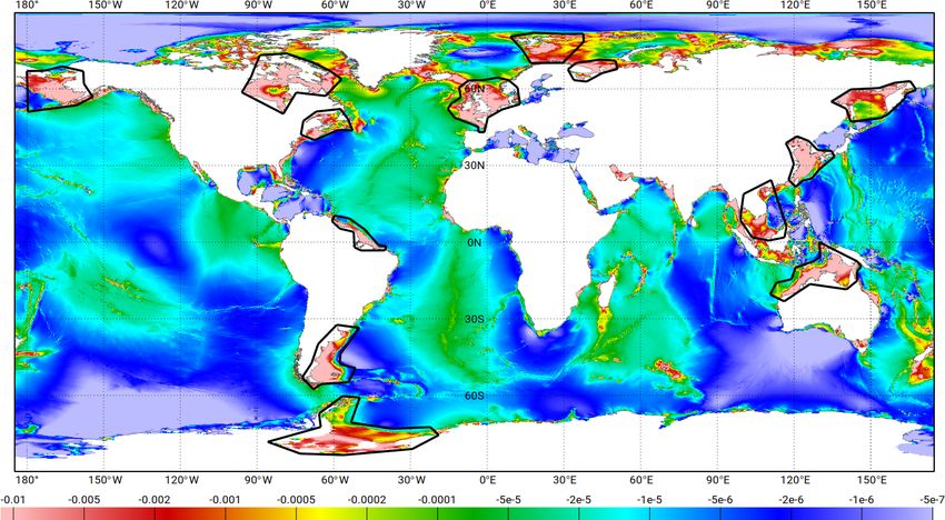
F. H. Lyard et al.: FES2014 global ocean tide atlas                                                                              619

form a macro-obstacle to the tidal propagation. Considering           racy is very limited on shelves and in coastal regions (Gibbs
the tedious task of remeshing most of the ocean shorelines,           effect due to the spherical harmonic technique, uncertain-
automated tools have been developed to optimize the mesh-             ties arising from sediment density, etc.) and consequently
ing operation. The targeted resolution for coastal areas is typ-      should not be used in such locations except in some spe-
ically 10 km or less in terms of triangle-side length (shown          cific areas, namely in the absence of any other more accurate
in Fig. 1; the mesh details will not be visible on a printed          bathymetry. It must be noticed that the latest GEBCO distri-
global ocean figure; the authors have provided a zoomable             butions now include patches derived from inverted bathyme-
Supplement .pdf file available on the Ocean Science website           tries, which is a serious issue for using recent GEBCO distri-
https://www.ocean-science.net/, last access: 28 March 2021).          butions in FES model bathymetry. Consequently, as for the
The resolution has been augmented to about 1.5 km in some             earlier FES atlases, a composite bathymetry has been built
specific places where coastal geometry is more challenging            from available global and regional databases. In some cases,
(such as fjords, estuaries, straits, etc.). Special attention was     a regional digital terrain model (DTM) has been specifi-
paid to regions where the accuracy and the precision of the           cally constructed from depth sounding and/or multi-beam
available bathymetry are known to be adequate with higher             data. A special treatment is applied to the Ross and Wed-
mesh resolution, i.e. where mesh details will truly reflect the       dell seas, where the free water column depth must be pro-
bottom topography complexity. On the other hand, only mi-             cessed by subtracting ice-shelf immersion to the bottom to-
nor upgrades were made in regions where the bathymetry re-            pography, using the RTopo-1 dataset (Timmermann et al.,
mains poorly known (such as the Patagonian and Siberian               2010). Many regions of the world ocean are now quite well
shelves). As a matter of experience, increasing resolution in         documented in terms of bathymetry; however, two major
those regions would likely have a model accuracy worsen-              continental shelves, namely the Patagonian shelf and the
ing effect. An additional constraint was to limit the hydrody-        Siberian shelf, do not match modern standards in any pub-
namic solver memory use to 30 GB in order to keep compu-              licly available database. Bathymetry selection, reconstruc-
tation load at a tractable level (at the time of production). De-     tion, and merging are tedious tasks, and they are quite un-
spite the large increase in resolution compared to FES2004,           certain because of the lack of independent validation data.
the FES2014 mesh resolution is still clearly not sufficient in        Finally, the most practical way to assess bathymetry changes
some highly complex coastlines, with narrow channels of dy-           remains the examination of the tidal solutions computed from
namical significance, or topographically trapped wave gen-            the candidate bathymetry. Naturally, this is not a perfect mea-
eration sites, and it could result in a loss of details/accuracy      sure of accuracy, as errors in bathymetry can compensate
in such regions. This is, for instance, the case of the west-         some other modelling errors, but so far we have always found
ern Canadian and Alaska coastal regions (where the project            consistent results between improvements in bathymetry and
failed to access any accurate bathymetry database at the time         tidal solutions. Thanks to the FD solver, extensive simula-
of production and so left resolution at a standard level), and it     tion testing can be performed, including the necessary recali-
has resulted in a loss of details/accuracy in all of this area, es-   bration loop needed when modifying significantly the model
pecially away from assimilated data. Following the FES2014            bathymetry, even on a regional level, as earlier calibration
atlas release and thanks to our collaboration with the Cana-          settings would be biased to compensate errors due to the
dian tidal research community, this issue has been identi-            former model bathymetry. Despite those efforts, bathymetry
fied as quite damaging. This issue and similar ones such as           still remains unfortunately the limiting error to our prior hy-
around the Tierra del Fuego (Argentina and Chile) will be             drodynamic solutions in most of the global ocean, and also
fixed in a future FES atlas release, where the number of com-         impacts the data assimilation accuracy in shallow-water re-
putational nodes should be increased at least by a factor of 5        gions. For most of North American, European, and Japanese
compared to the FES2014 grid.                                         waters, bathymetry-linked errors are reducing with time, al-
                                                                      lowing for distinguishing more subtle error sources. For in-
2.5   Model bathymetry                                                stance, thanks to the impressively accurate new bathymetry
                                                                      of the European shelf (as available through the European
When dealing with tides, bathymetry remains one of the                Marine Observation and Data Network (EMODnet) website,
most critical parameters. Several global ocean databases              https://emodnet.eu/en, last access: 28 March 2021), most of
were available at the FES2014 production time: the General            errors due to bathymetry have been dramatically reduced, so
Bathymetric Chart of the Oceans (GEBCO, GEBCO compi-                  we could clearly demonstrate (in a regional configuration)
lation group, 2020), Earth Topography (ETOPO; Amante and              that a wetting–drying time-stepping scheme is necessary to
Eakins, 2009), Smith and Sandwell (Smith and Sandwell,                reach the best tidal accuracy in the North Sea. Using older
1997), etc. Their successive releases have shown tremendous           bathymetry would have totally blurred this point, making
improvements during the last 10 years. Unfortunately, none            any conclusions uncertain. But in most of the global ocean,
of those global databases have the effective resolution or the        improving the model bathymetry remains the first and over-
accuracy needed to be used directly in our global ocean tides         whelming priority, and enormous efforts have been dedicated
modelling. For example, satellite-inverted bathymetry accu-           to this in FES2014 hydrodynamic configuration settings.

https://doi.org/10.5194/os-17-615-2021                                                              Ocean Sci., 17, 615–649, 2021
620 F. H. Lyard et al.: FES2014 global ocean tide atlas
2.6 Loading and self-attraction effects improvement that has been achieved from the FES2004 to
the FES2014 free simulations on the global ocean, with a
Geometrical loading and gravitational self-attraction (LSA) global vector difference root mean square (rms) reduced by
terms are essential in tidal simulations, especially in global nearly a factor of 3 from FES2004 to FES2014 (M2 tidal
ocean tidal modelling (Hendershott, 1972). They can be im- component) in the deep ocean. The improvements are also
plicitly accounted for in the hydrodynamic tidal equations very strong in the shelf regions and for the other main tidal
but at a totally prohibitive computational cost. As rather ac- components. Moreover, the histograms displayed in Sect. 5.2
curate LSA atlases have been available since the early 2010s, indicate that the FES2014 hydrodynamic solution reaches an
it is much more efficient to use explicit LSA in the simula- unprecedented accuracy level, close to other global ocean
tions, not only for computational cost reasons (non-sparse model performance as such GOT4.8/10 (Ray, 2013), EOT11a
dynamical matrices in FD, expensive convolutions in LSA (Savcenko and Bosch, 2012), DTU10 (Yongcun and Ander-
computation) but also because it tends to provide a relax- sen, 2010), or TPXO9v2 (Egbert and Erofeeva, 2002), which
ation toward the tidal atlases from which the LSAs have been are all empirical or assimilated models.
computed (actually, this is the only model ingredient which The case of the S2 tidal components was specifically ad-
depends upon pre-existing ocean tide information in our hy- dressed, as it derives both from atmospheric and gravitational
drodynamic simulations). As some anomalies were detected forcing. It is even more the case for the S1 tide, which origi-
in the LSA atlases deduced from FES2004, we used instead nates mostly from atmospheric forcing, but because of the in-
the FES99-derived LSA atlases to produce a first version trinsic variability of the atmosphere we consider that it must
of FES2014 (FES2014a), from which a new LSA atlas was be dealt with in the storm surge correction (dynamic atmo-
computed. As will be mentioned in the following sections, spheric correction; DAC) and not in ocean tidal corrections.
this new LSA atlas was used in the final FES2014b release Some other tidal constituents have a clearly atmospherically
production. forced component (such as K2 and even M2 tides) but at a
much lower level. Consequently, to ensure the best possi-
2.7 FES2014 hydrodynamic (assimilation-free) ble prior solution, the S2 wave was computed in the spec-
solutions tral domain using atmospheric pressure forcing at S2 fre-
quency, based on ERA-Interim 3 h data (Berrisford et al.,
Some parameters of the T-UGOm hydrodynamic model need 2011). There are numerous difficulties arising from the at-
to be calibrated in order to obtain the most accurate hydro- mospheric pressure forcing at tidal frequencies (impacting
dynamic solution, either to improve model realism or pro- tidal hydrodynamic solutions, de-aliasing corrections, and
vide useful error compensation. The two main parameters data processing), so additional discussions on S1 and S2 con-
to which the model is most sensitive are the bottom fric- stituent issues are given in the following sections.
tion coefficient and the internal tide drag coefficient. Most of
T-UGOm model parameters can optionally be tuned locally
using various methods (pre-defined regions, polygons inclu- 3 Tidal harmonic constant data processing
sion, or by mesh node or element vectors). In the FES2014
atlas simulations, internal wave drag coefficients are tuned TG and altimetry-derived harmonic constant data have been
using a global ocean regional partition (distinguishing north, used in validation of simulations and data assimilation steps.
tropical, and south basins in the various oceans plus the Arc- Concerning the TG data, preference was given to TGs for
tic Ocean and Mediterranean Sea), and bottom friction coeffi- which the original time series were available and docu-
cients are tuned by using polygons covering the large bottom mented, and hence for which basic quality control could be
friction dissipation areas. A global default value is locally performed by means of harmonic analysis and/or operational
used in regions not being targeted by the user-defined parti- reports. In most cases, the time series were long enough
tion/polygon tuning list. Several simulations of the main tidal so that a wide tidal spectrum could be analysed with the
components (limited to M2, K1, S2, and O1 constituents) best possible accuracy. To some extent, TG selection (ei-
have been performed by extensively varying these two pa- ther for validation or data assimilation purposes) is more a
rameters (mostly globally except in a few regions for the question of how representative the tides captured by the in-
internal tide drag coefficient), and each resulting simulation struments are (especially in coastal seas) and keeping a bal-
was compared to the altimetry and tide gauge (later denoted anced distribution all over the ocean regions. Several tidal
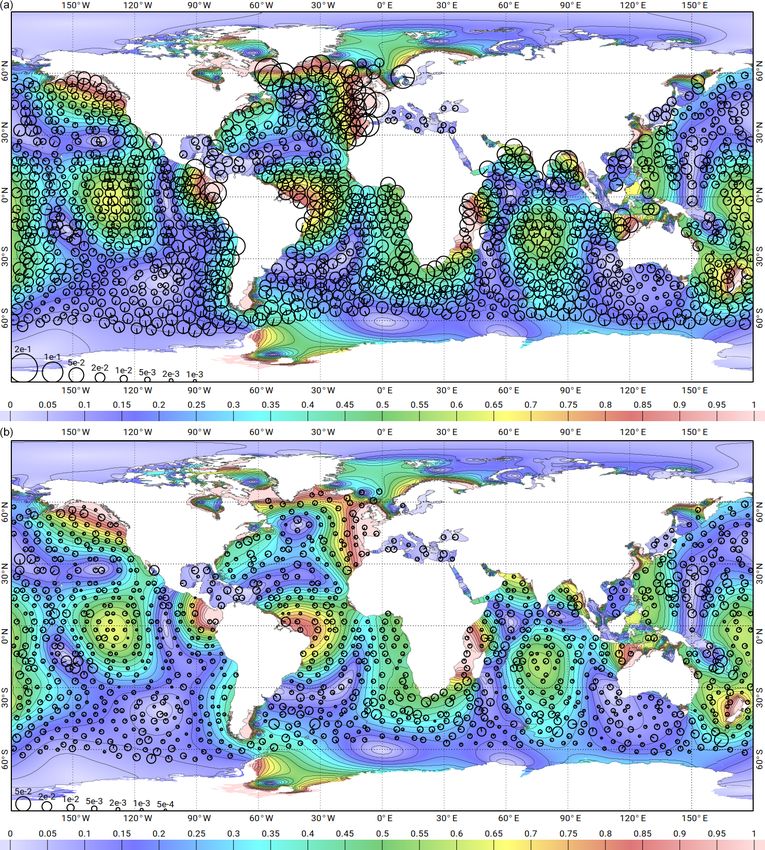
TG) validation databases. Figures 2 and 3 show the vec- gauge databases have been used within the FES2014 project:
tor differences between the TP/J1/J2 (deep ocean) crossover a harmonic analysis was performed on time series from the
point database and the hydrodynamic simulations of the GLOSS (Holgate and al., 2013) and SONEL (Wöppelmannn
FES2012 and FES2014 tidal models, for the M2 and K1 and Marcos, 2015) databases, GLOSS being a global obser-
tidal components, respectively. Global values of vector dif- vation network and SONEL providing measurements on all
ferences are given in Table 1 for the same two hydrodynamic French territories; then, three validated databases provided
simulations plus FES2004. These results clearly point out the by R. Ray have been used (Ray, 2013), named Deep_BPR
Ocean Sci., 17, 615–649, 2021 https://doi.org/10.5194/os-17-615-2021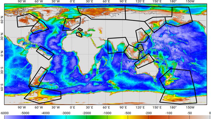
F. H. Lyard et al.: FES2014 global ocean tide atlas                                                                                  621

Figure 2. Vector differences (black circles) between the purely hydrodynamic solutions of FES2012 (a) and FES2014 (b), and the deep
TP/J1/J2 altimeter crossover points, for the M2 tidal component. The accuracy improvement between the FES2012 and FES2014 prior
solutions is a key ingredient in the accuracy improvement between the FES2012 and FES2014a/b/c assimilated solutions. The size of the
black circles is proportional to the square root of the amplitude of the vector difference between the solutions and the observations (see
bottom left normalized symbols; units are in metres). The line inside circles shows the vector difference phase. The background colour
shows the amplitude of the M2 tidal component from the model (in metres).

(bottom pressure recorders), Shallow, and Coastal, hereafter              The altimetry-derived time series raise more processing
and dedicated to deep ocean, shallow waters, and coastal re-           and accuracy issues, with a strong dependence on the mis-
gions, respectively.                                                   sion orbit and duration (which firstly determine the level
                                                                       of contamination of the tidal analysis by non-tidal ocean

https://doi.org/10.5194/os-17-615-2021                                                                 Ocean Sci., 17, 615–649, 2021
622                                                                           F. H. Lyard et al.: FES2014 global ocean tide atlas

Table 1. The rms of the vector differences (in cm) between the purely hydrodynamic solutions of FES2004, FES2012, and FES2014, and the
TP/J1/J2 altimeter crossover points, for the M2 and K1 tidal components. The accuracy improvement between the FES2012 and FES2014
prior solutions is a key ingredient in the accuracy improvement between the FES2012 and FES2014a/b/c assimilated solutions.

                                           M2 tidal component                                      K1 tidal component
                            Crossover TP/J1/J2 deep    Crossover TP/J1/J2 shelf    Crossover TP/J1/J2 deep   Crossover TP/J1/J2 shelf
 FES2004 hydrodynamic                          4.56                        12.32                      1.45                      4.19
 FES2012 hydrodynamic                          2.38                         9.25                      1.07                      2.97
 FES2014 hydrodynamic                          1.53                         6.44                      0.88                      2.26

signals). Clearly, the 20-year and longer duration of the            vent us from using ERS/Envisat-derived data and concen-
TOPEX/Poseidon (TP) and Jason series on a nearly 10 d                trate only on the TOPEX/Jason dataset; however, the incli-
repeat orbit allows for deriving outstandingly high-quality          nation of TOPEX/Jason is rather low and ERS/Envisat re-
along-track and crossover datasets of tidal harmonic con-            mains the only choice for very high latitudes and polar seas.
stants (TOPEX/Poseidon, Jason-1 (J1), and Jason-2 (J2) are           Thus, for the purpose of the FES2014 tide model, crossovers
three CNES/NASA satellites, successively launched, having            and along-track data from TOPEX/Jason-1/Jason-2 were pre-
exactly the same ground track and repetitivity, and simi-            ferred and were complemented with some crossover data
lar on-board instruments and radar technologies. Since the           from TPN/J1N and ERS/Envisat series in some shallow-
FES2014 release, the series has been continued with the              water regions and at high latitudes, respectively. Table 3
Jason-3 and Jason-CS satellites; at the end of their nominal         presents the altimeter dataset used for the estimation of the
missions, a satellite’s orbit is changed toward an exactly in-       harmonic constants within the FES2014 project.
terleaved ground track, hence doubling the mission spatial
sampling until a possible move to a geodetic orbit or final de-      3.1    Tidal loading effect
commissioning. Interleaved track observations are not con-
tinuous in time and thus have shorter records compared to            As the standard tidal atlases are targeted on the ocean tide
the nominal track records). Moreover, the altimetry dataset          component, a tidal loading correction needs to be applied to
benefits from new altimeter standards, which allow a better          the altimeter measurements (in addition to the so-called solid
observation of the tidal signals: GDR-D and REAPER orbits,           Earth deformation correction). In a first step, the GOT4v8ac
ERA-Interim DAC for the European Remote-Sensing Satel-               tidal loading model was applied (Ray, 2013), taking into
lite (ERS) and TOPEX missions, improved wet tropospheric,            account the recent correction of the tidal geocentre motion
sea sate bias, and ionospheric corrections, and new mean sea         proposed by Desai and Ray (2014). These data have been
surface profiles computed over a 20-year period (Carrère and         used in the data assimilation process for the preliminary ver-
Lyard, 2003; Carrere et al., 2016). The TOPEX-interleaved            sion of the ocean tide model, denoted FES2014a. In a sec-
and Jason-1-interleaved track (denoted TPN/J1N) also pro-            ond step, a new tidal loading atlas was computed from this
vides an accurate crossover dataset but with larger uncer-           FES2014a ocean solution, denoted “FES2014a tidal loading”
tainties than the 20 years of TOPEX/Jason series, due to the         (see Sect. 6.3). Then, this FES2014a tidal loading solution
shorter cumulative period of 6 years available. ERS/Envisat          was used to produce a second version of the altimeter dataset,
series and Geosat Follow-On (GFO) series do not have the             which was assimilated into the final version of the tide model
same level of accuracy, as their orbits offer higher spatial         named FES2014b.
coverage at the price of a lower temporal coverage (time
                                                                     3.2    Prior removal of the non-tidal signal at the K1
sampling of 35 d for ERS/Envisat and 17 d for GFO). The
                                                                            aliased period
temporal undersampling of tidal observations affects the ap-
parent tidal periods (aliasing effect) which depend on the           Due to the aliasing effect, the K1 diurnal frequency is aliased
true tidal periods and on the mission temporal repetitivity.         to the semi-annual frequency with the TOPEX/Jason sam-
Because of the red nature of the ocean energy spectra, the           pling and to the annual frequency with the ERS/Envisat orbit
longer the aliased period, the larger the contamination of           (see Table 2). Annual and semi-annual signals are quite large
the tidal signal by non-tidal signals. The TOPEX/Jason orbit         in the ocean, and contamination of tidal analysis by the non-
was deliberately chosen to maintain the aliased period in a          tidal signal is severe. By virtue of the Parseval identity (the
reasonable range. Conversely, Sun-synchronous orbits (such           identity asserts that the sum of the squares of the Fourier co-
as ERS/Envisat/AltiKa) are disadvantageous in that matter:           efficients of a function is equal to the integral of the square
not only are the S1 and S2 tides projected on an infinite pe-        of the function; see Johnson and Riess, 1982), this contami-
riod (mean state), but many other tidal constituents show a          nation decreases with time as the square root of the record-
rather large aliased period (see Table 2). This would pre-           ing duration. The present reference TOPEX/Jason time se-

Ocean Sci., 17, 615–649, 2021                                                              https://doi.org/10.5194/os-17-615-2021
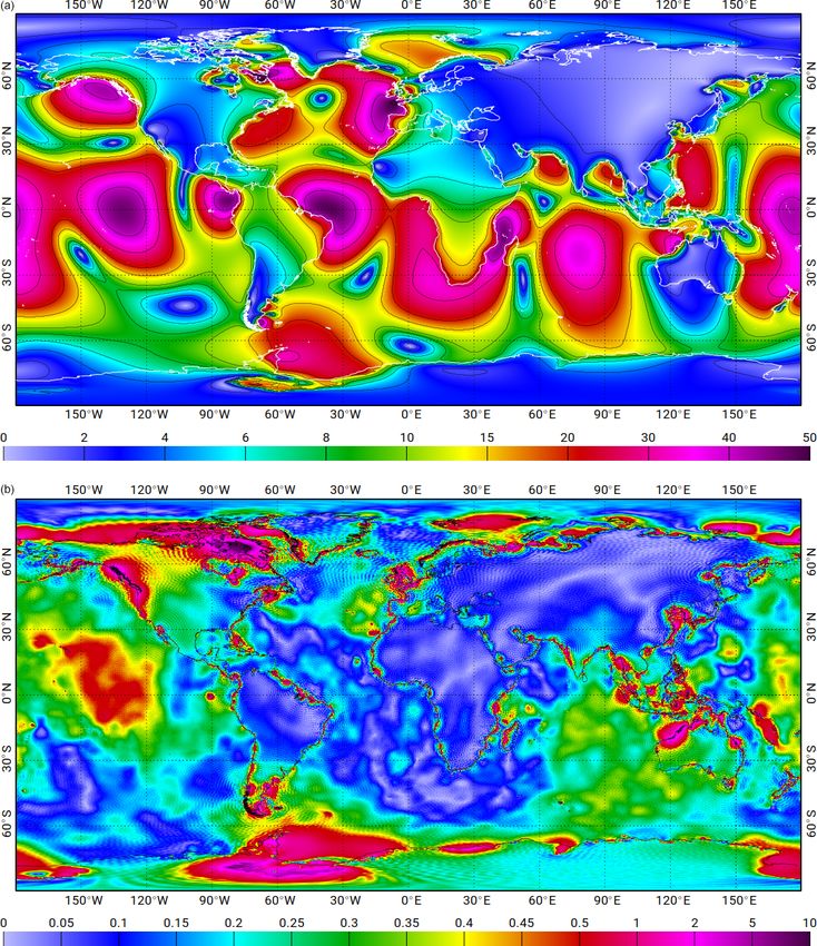
F. H. Lyard et al.: FES2014 global ocean tide atlas                                                                                  623

Figure 3. Vector differences (black circles) between the purely hydrodynamic solutions of FES2012 (a) and FES2014 (b), and the deep
TP/J1/J2 altimeter crossover points, for the K1 tidal component. The accuracy improvement between the FES2012 and FES2014 prior
solutions is a key ingredient in the accuracy improvement between the FES2012 and FES2014a/b/c assimilated solutions. The size of the
black circles is proportional to the square root of the amplitude of the vector difference between the solutions and the observations (see
bottom left normalized symbols; units are in metres). The line inside circles shows the vector difference phase. The background colour
shows the amplitude of the M2 tidal component from the model (in metres).

ries benefits from 20 years of continuous measurements and             antee an accurate separation of the K1 tidal signal from the
allows a very accurate estimation of all tidal components in-          semi-annual (annual) ocean variability. A large portion of the
cluding K1. However, for the TPN interleaved and the ERS               annual and semi-annual ocean surface signal is due to the
orbits, the available time series are not long enough to guar-         low-frequency atmospheric surface pressure and therefore is

https://doi.org/10.5194/os-17-615-2021                                                                 Ocean Sci., 17, 615–649, 2021
624                                                                                 F. H. Lyard et al.: FES2014 global ocean tide atlas

Table 2. Aliasing periods of main tidal waves for TOPEX/Jason, ERS/EN, and GFO altimeter samplings.

                                                        Satellite name         TP/Jason             GFO     Envisat ERS-2
                                                 Satellite cycle (days)          9.9156          17.0505               35
                                     Darwin               True period     Aliased period   Aliased period   Aliased period
                                     name                      (days)             (days)           (days)           (days)
                   Long-period       Ssa                       182.62             182.62          182.62           182.62
                   tides             Mm                        27.554             27.554          44.727           129.53
                                     Mf                        13.661             36.167          68.714           79.923
                   Diurnal           Q1                        1.1195             69.364          74.050           132.81
                   tides             O1                        1.0758             45.714          112.95           75.067
                                     P1                        1.0027             88.891          4466.7           365.24
                                     K1                        0.9972             173.19          175.45           365.24
                   Semi-diurnal      N2                        0.5274             49.528          52.072           97.393
                   tides             M2                        0.5176             62.107         317.108           94.486
                                     S2                        0.5000             58.741          168.82               ∞
                                     K2                        0.4986             85.596          87.724           182.62

Table 3. Description of altimeter data used.                                the NEMO model forcing and are corrected for in the assim-
                                                                            ilated sea surface height (SSH) data). Consequently, they are
                          TP/J1/J2    TPN/J1N               ERS/EN          comparable to inverted barometer (IB) corrected sea level (at
  Min/max latitude        ±66.14◦     ±66.14◦      80.25◦ N/75.44◦ S        Sa and Ssa frequencies) in altimetry and tide gauge observa-
  Cycle duration (days)   9.91564      9.91564                   35         tions. GLORYS2v1 SSH has been harmonically analysed at
  Number of cycles used       743          223                  172         semi-annual and annual frequencies, predicted at observation
                                                                            location and time and removed from altimetric SSH measure-
                                                                            ments. The efficiency of the non-tidal ocean signal contami-
                                                                            nation has been assessed at TOPEX/Jason crossovers, where
removed by applying a storm surge or inverted barometer                     the K1 harmonic constant misfits between ascending track
correction. However, the ocean circulation contributes also to              and descending track analysis are diminished. As shown in
this signal, and so to tidal harmonic contamination. To tackle              Fig. 4, the amplitude of the correction is well above a few
this issue, and then improve the K1 tidal signal observation                centimetres in some large ocean regions. A specific study
in the TPN and ERS/Envisat records, a specific processing                   (Gulf of Tonkin) was performed by examining the K1 anal-
has been applied, consisting in removing an estimation of the               ysed tidal constant misfit at crossovers (ascending track ver-
ocean annual (Sa) and semi-annual (Ssa) non-tidal signals                   sus descending track). The ocean circulation contamination
prior to the analysis. This estimation is computed from the                 will appear as an incoherent contribution to K1 and will be
Global Ocean Reanalysis and Simulations (GLORYS) 2v1                        different for ascending and descending tracks. Such differ-
global ocean reanalysis provided by Mercator Ocean (Ferry                   ences were found to be consistently reduced when applying
et al., 2012). GLORYS produces and distributes global ocean                 the GLORYS correction, hence demonstrating the benefits of
reanalyses at eddy-permitting (1/4◦ ) resolution that aim to                the model-based correction for the tidal analysis accuracy.
describe the mean and time-varying state of the ocean cir-
culation, including a part of the mesoscale eddy field, over                3.3   S2 tidal constituent processing
recent past decades with a focus on the period since when
satellite altimetry measurements of sea level provide reli-                 S2 tide harmonic analysis needs a special attention both
able information on ocean eddies (i.e. from 1993 to present).               in TG and altimetry time series. Because of the significant
The numerical model used is the Nucleus for European Mod-                   S2 atmospheric tide, especially in the tropics, bottom pres-
elling of the Ocean (NEMO) ocean general circulation model                  sure records must be precisely corrected from air pressure
(OGCM) in the ORCA025 configuration developed within                        contribution to retrieve the S2 ocean signal. This is easily
the DRAKKAR consortium (global with sea ice, 1/4◦ Mer-                      done for coastal TGs, from dedicated or neighbouring atmo-
cator grid). Assimilated observations are in situ temperature               spheric pressure records. Deep moorings in remote ocean re-
and salinity profiles, satellite sea surface temperature (SST)              gions are more problematic, especially for records made be-
and along-track sea-level anomalies obtained from satellite                 fore the quite recent availability of hourly pressure fields in
altimetry. GLORYS2v1 products are free of atmospheric sur-                  operational atmospheric products. In altimetry mission ob-
face pressure effects (i.e. they are not taken into account in              servations, the S2 tidal constituent is challenging as it is

Ocean Sci., 17, 615–649, 2021                                                                    https://doi.org/10.5194/os-17-615-2021
F. H. Lyard et al.: FES2014 global ocean tide atlas 625 Figure 4. Maps of amplitude in metres of Sa (a) and Ssa (b) ocean signals estimated from GLORYS2v1 reanalysis. GLORYS2v1 products are free of atmospheric surface pressure effects (i.e. they are not taken into account in the NEMO model forcing and are corrected for in the assimilated SSH data). Consequently, they are comparable to IB-corrected sea level (at Sa and Ssa frequencies) in altimetry and tide gauge observations. aliased to infinite period and thus is not observable by the ble at the same frequency in the TOPEX/Jason time series, ERS/Envisat Sun-synchronous orbit as mentioned before. which in turn is linked to inaccuracy in the β 0 angle in MSL The TOPEX/Jason orbit is adequate for the observation of computations (Zawadzki et al., 2018). Consequently, S2 har- most of the main tidal constituents. However, because of monic analysis will be contaminated by this geophysical data its 58.74 d aliased period, the S2 tide sea surface signal is record (GDR) processing-dependent signal (with a possible mixed with the residual mean sea level (MSL) signal visi- feedback through the tidal corrections in the GDRs, mak- https://doi.org/10.5194/os-17-615-2021 Ocean Sci., 17, 615–649, 2021
626                                                                      F. H. Lyard et al.: FES2014 global ocean tide atlas

ing this issue even more complicated). As this problem is         examined the ratio between the diagonal and extra-diagonal
larger for the TOPEX/Poseidon mission GDRs (as reported           terms in the numerical harmonic matrix, and we used an anal-
in Zawadzki et al., 2018), several analyses have been per-        ogy with the Rayleigh criterion for continuous time series
formed using either the entire TOPEX/Jason time series or         (and the corresponding harmonic matrix) to decide on a max-
only the Jason-1/Jason-2 relatively recent records. But due       imum ratio (extra-diagonal / diagonal) above which the fre-
to the much shorter duration of the latter, the estimation er-    quency separation was considered deficient. The maximum
ror is larger for the J1/J2-only analysis, and the assimilated    ratio is set by analogy with the Rayleigh criterion. Ideally,
solution proved finally to be more accurate (using TG data        i.e. in the case of quasi-infinite time series, the harmonic
as sea truth) using the analysis from the entire altimeter se-    matrix will be quasi-diagonal. The shorter the time series,
ries. Notice that thanks to its primary emphasis on accurate      the larger the cross-term / diagonal-term ratio in the matrix,
hydrodynamic modelling, further moderately tuned by data          which reflects the loss in separation efficiency. In the case of
assimilation (thus allowing a reduced weight of the data and      a regularly sampled continuous time series (no data missing),
data errors in the global FES solution), the FES2014 S2 so-       the usual Rayleigh criterion (at least one period difference
lution is less affected by this residual GDR processing signal    between two different constituents over the time series dura-
than empirical models, with in addition a beneficial effect on    tion) is equivalent to a maximum ratio of ∼ 0.15 in any row
reducing the residual MSL error if used for tidal corrections     of the harmonic matrix. In the case of two constituents show-
in GDR processing (Zawadzki et al., 2018).                        ing a ratio larger than 0.15, we check whether admittance can
                                                                  be used to infer the one with the lowest astronomical poten-
3.4   Numerical Rayleigh criterion                                tial or not. If this is not the case or if at least one is a non-
                                                                  astronomical constituent, it is dismissed from the harmonic
When extracting a comprehensive tidal spectrum from a sea-        analysis spectrum.
level time series, the question of frequency separation must
be examined carefully (Cherniawsky et al., 2001). Not only        3.5   Filtering internal tide signatures
can the contamination by non-tidal signals at the aliased
frequency be comparable to a given constituent amplitude          FES2014 is a barotropic tide model and it is not aimed to
(especially the minor constituents), but also the minimum         include the small scales of the internal tide signals by defi-
observation duration for a proper separation is greatly in-       nition. Thus, internal tide surface signatures have to be re-
creased in the aliased frequency space. For instance, the N2      moved from the altimeter data prior to data assimilation
and T2 pair needs about a minimum of a 7-year duration in         and validation processes. Internal tides have much shorter
TOPEX/Jason observations) for a proper separation instead         wavelength (and much lower phase speed) than barotropic
of the usual 10 d in the non-aliased frequency space. The data    tides, and their juxtaposing with barotropic tides creates well
assimilation spectrum in FES2014 is a mitigation between          known ripples in the along-track harmonic analysis due to
the objectives of extending the tidal correction spectrum and     in-phase/out-of-phase changes (Egbert and Ray, 2001). So
limiting data assimilation to accurately observable tidal con-    low-pass filtering is a convenient way (still imperfect as it
stituents, and we have developed a new numerical approach         is vulnerable to the baroclinic waves propagation angle with
to address the frequency separation issue. In the case of a       respect to the ground track) to separate barotropic and baro-
continuous (i.e. uninterrupted or sparsely interrupted) time      clinic tide components for each frequency. Based on gravity
series, the Rayleigh criterion is classically used to determine   wave vertical modes theory (Gill, 1982), new estimates of the
frequency separation, and some additional parameterization        first vertical mode, baroclinic wavelengths have been com-
(based on the smoothness credo or admittances) can be im-         puted for the main waves (M2, N2, S2, K1, and O1) using
plemented to ease the harmonic system solving. For TGs            WOA2009 climatology (Locarnini et al., 2010, Antonov et
as well as for most of the altimetry-derived time series, the     al., 2010). First-mode baroclinic tides show the largest wave-
Rayleigh criterion will be appropriate to predict rather ac-      lengths, which are roughly in the 100 to 150 km range in the
curately the harmonic separation performance. However, in         deep ocean and much shorter on shelf seas. Still, barotropic
the case of high-latitude altimetric time series, the seasonal    tides have short wavelength in their amplitude and phase
sea ice cover is responsible for annually unbalanced observa-     distribution, for instance, close to amphidromic points or
tions, with data gaps duration that can be comparable to the      at shelf edge crossing, that should not be filtered out. The
aliased wave frequency. In that case, it has been observed that   barotropic tide wavelength has been numerically computed
the Rayleigh criterion will return over-optimistic diagnostics.   from the FES2012 atlas (by estimating the local wavenum-
This turns into an ill-defined harmonic system and conse-         bers from the ratio of the complex Laplacian of the tidal
quently larger errors in the harmonic constants deduced from      elevation field and the tidal elevation field itself), and both
its solving. Neither high-latitude dataset manual editing nor     barotropic and baroclinic estimates were then used to com-
entire dataset rejection were options, the former being a gi-     pute the along-track low-pass-filtering cutting length scale,
gantic task and the latter an extremely damaging loss of data     which is the minimum between twice the baroclinic wave-
in already poorly documented regions. Instead, we directly        length and 1/15th of the barotropic one. Figure 5 shows the

Ocean Sci., 17, 615–649, 2021                                                          https://doi.org/10.5194/os-17-615-2021
F. H. Lyard et al.: FES2014 global ocean tide atlas 627
Figure 5. Along-track filtering wavelength used to remove internal tides’ surface signatures (expressed in number of 1 Hz along-track points,
to be multiplied by a factor of 6 to retrieve the equivalent wavelength in kilometre).
filtering cut-off length scale in kilometres: it goes to zero in quite well designed to capture model errors arising from the
near-amphidromic point areas and in shallow waters where right-hand side of the tidal equations (linear forcing terms), it
the wavelength of the barotropic tide becomes shorter. turns to be poorly able to account for bathymetry-derived and
non-linear terms (bottom friction) errors that usually domi-
nate modelling errors in coastal and shelf seas. For this rea-
4 Data assimilation son, an ensemble approach has been constructed to improve
the realism and flexibility of the modelling error prescrip-
The data assimilation method used in FES2014 is quite sim- tions. The optimal interpolation denomination is a misnomer
ilar to the one used in FES2004, with the notable excep- as the error covariances of the state vector are not idealized
tion that the ensemble approach has been substituted by the covariances (such as Gaussian-shaped distribution) but are
variational one. This change in our approach, initiated after justified by the non-incremental nature of the data assimila-
FES2004 completion, is motivated by the difficulty to pre- tion due to the frequency-domain space where it applies.
scribe bathymetry errors as right-hand side, forcing terms er-
rors, as a variational technique would ask for. More gener-
4.2 Ensemble construction
ally, the ensemble technique is much more flexible and natu-
ral, especially when dealing with highly inhomogeneous er-
ror sources, in nature and magnitude, as is the case for shelf In the ensemble assimilation approach, a large number of
and coastal tides. simulations are run in order to describe the model errors.
This ensemble of simulations is generated by varying the pa-
4.1 SpEnOI assimilation code rameters and input datasets to which the model is the most
sensitive. In the case of the FES2014 tidal model, the per-
The SpEnOI (Spectral Ensemble Optimal Interpolation) data turbations were made on the bottom friction coefficient, the
assimilation code is an evolution of the Code d’Assimilation internal tide drag coefficient, the bathymetry and the LSA.
Océanique par la méthode des Représenteurs (CADOR) data All the simulations were validated against the altimetry and
assimilation code (Lyard, 1997, used up to FES2004), based the TG databases, in order to identify potential outliers. In
on a variational approach using a representer method, orig- addition, the dispersion of the ensembles and the distance
inally inspired by Bennett and MacIntosh (1982). The main of the ensemble mean to the reference hydrodynamic simu-
difference lies in the fact that CADOR uses a variational for- lation were computed, in order to verify that the ensembles
mulation to infer the tidal elevation error covariance matrix, were centred on the reference. In total, the whole ensemble
using an adjoint system. Although the variational approach is contains 432 simulation members for each tidal constituent,
https://doi.org/10.5194/os-17-615-2021 Ocean Sci., 17, 615–649, 2021628 F. H. Lyard et al.: FES2014 global ocean tide atlas
Figure 6. Energy (W m−2 ) dissipated by bottom friction in the FES2014 hydrodynamic model, for the M2 wave, and polygons used for the
perturbations of the bottom friction coefficient.
built by following the methodology described in the next sec- get back at least to a similar or improved accuracy. In order
tions. to obtain a thorough description of the model errors, all the
simulations based on perturbations were done twice, using
4.2.1 Perturbation of the loading tide the FES99 and the FES2012 loading tides as input, respec-
tively. This doubled the number of members in the ensembles
Numerical experiments have shown that the model is very described hereinafter.
sensitive to the explicit LSA forcing, with tidal species de-
pendence. Namely, the diurnal tidal components (K1, O1) are 4.2.2 Perturbation of the bottom friction roughness
improved when using the FES2012-derived LSA, while the
semi-diurnal tidal components (M2, S2) are better resolved
when using the FES99-derived LSA. The latter result needs Figure 6 shows the energy dissipated by the bottom friction
some explanations: first, the FES2014 hydrodynamic config- in the FES2014 hydrodynamic model for the M2 tidal com-
uration has been adjusted (i.e. bottom friction and internal ponent. As expected, the areas where the dissipation is the
wave drag due to barotropic to baroclinic energy conversion, largest correspond to the shelves and coastal seas. The model
denoted IWD) in simulations using the FES99 LSA, and in- is consequently more sensitive to the bottom friction coeffi-
cluding clearly an error compensation contribution, i.e. con- cient in these areas. Following this map, 13 polygons, high-
figuration adjustments compensate for the FES99 LSA de- lighted in red in Fig. 6, were defined in order to generate lo-
fects. Consequently, considering the high level of accuracy cal perturbations of the bottom friction coefficient in signif-
of the hydrodynamic solutions and thus the sensitivity to any icant bottom friction tidal dissipation regions. The definition
minor changes, they are not fully appropriate for a simula- of tuning polygons is a compromise to include the most sig-
tion forced with another LSA atlas; second, the most sen- nificant sites for tidal dissipation and to limit the number of
sitive component in the adjustment process is clearly M2, polygons (to avoid too many members in our ensembles). For
as bottom friction is truly non-linear for M2, as it has the each of these polygons, the bottom friction roughness was
strongest currents and the dominates the velocity amplitude assigned eight different values ranging around the global-
in the non-linear friction term, and as the other constituents average value set for the reference hydrodynamic simulation
have consequently a kind of quasi-linear friction in the pres- (10−3 m). As presented above, all the simulations were done
ence of M2 dominant velocities. So using a more modern twice, with the FES99 and the FES2012 loading tides, re-
and more accurate LSA will usually profit all constituents but spectively, as input, and the ensemble of bottom friction per-
M2, as it would require reprocessing the adjustment steps to turbations finally contained 208 members.
Ocean Sci., 17, 615–649, 2021 https://doi.org/10.5194/os-17-615-2021F. H. Lyard et al.: FES2014 global ocean tide atlas 629
Figure 7. Divisions used for the perturbations of the wave drag coefficient.
4.2.3 Perturbation of the wave drag coefficient in Fig. 8 and chosen either for their dynamical impact on
tidal solutions or for the large uncertainties of the reference
Contrary to the bottom friction, the energy dissipation due bathymetry quality (such as the Patagonian shelf). However,
to the energy transfer from the barotropic tides to the baro- the construction of the ensemble simulations has highlighted
clinic tides (internal tide drag) does not happen in very spe- that the two bathymetry perturbations in the Weddell Sea
cific and local regions but in various dispersed, sloping bot- (southern Atlantic Ocean) resulted in solutions showing er-
tom topography regions (shelf edges, ocean ridges) where the rors in semi-diurnal tides up to 2–4 times larger than the av-
tidal currents cross the bathymetry gradients, making it diffi- erage simulations, with a large increase of errors in the whole
cult to isolate each individual active site. In addition, energy Atlantic Ocean, in the Indian Ocean and in the southern Pa-
transfer efficiency strongly depends on local ocean stratifi- cific Ocean. This comes from the free water depth reduction
cation, which is not precisely known in standard climatol- due to the Weddell Sea ice-shelf immersion, which has been
ogy or OGCMs. The perturbations of the wave drag coeffi- corrected in our reference bathymetry, but not in the gridone
cient were consequently done at the subdivided basin scale and Smith and Sandwell patches because of project sched-
(equatorial/tropical, midlatitude, and high-latitude subdivi- ule constraints. Despite being considered as potentially crit-
sions), shown in Fig. 7. For each of these 10 regions, the non- ical for the model error space, the Weddell Sea region was
dimensional wave drag coefficient was locally varied over discarded from the bathymetry patch ensemble construction,
seven values ranging around the global-average value set for whose effective set contains 36 members.
the reference hydrodynamic simulation (i.e. 75). The wave A few additional members have been added from the per-
drag perturbations ensemble finally contains 140 members turbations of the model minimal depth threshold. It is usu-
(70 perturbations run with each of the FES99 and FES2012 ally set to 10 m in the T-UGOm hydrodynamic global ocean
LSAs). model. Depth threshold aims to minimize frequency-domain
modelling validity limitations in very shallow waters (T-
4.2.4 Perturbation of the model bathymetry UGOm has the ability to modulate the threshold as a function
of local tidal range; it was not used in FES2014 to avoid ad-
Several approaches are possible for the hydrodynamic model ditional complexity in the model configuration setting) but
bathymetry perturbations, such as linear combinations of var- more importantly to deal with the existence of unrealisti-
ious datasets or modifications in specific regions using ei- cally shallow depths in most bathymetry datasets. The depths
ther synthetic or heterogeneous bathymetry dataset. The lat- found in most bathymetry databases in the 0–10 m (and prob-
ter was used in the case of the FES2014 model, as it en- ably 0–20 m) range are anything but reliable. In most places,
ables to better control the perturbations and to choose the the depths linearly vary with distance from 0 m at coastline
most responsive regions. The reference hydrodynamic model to the 10 m isobaths, which is not the usual morphology one
bathymetry is replaced by depths extracted from what we call will find in the true ocean. Such artificial, very-shallow-water
“gridone”, 1 min resolution from GEBCO, and Smith and patches can have a damaging impact on the bottom friction
Sandwell, 15.1 release, in each of the 19 regions displayed
https://doi.org/10.5194/os-17-615-2021 Ocean Sci., 17, 615–649, 2021You can also read