El Niño-Southern Oscillation signal in a new East Antarctic ice core, Mount Brown South
←
→
Page content transcription
If your browser does not render page correctly, please read the page content below
Clim. Past, 17, 1795–1818, 2021
https://doi.org/10.5194/cp-17-1795-2021
© Author(s) 2021. This work is distributed under
the Creative Commons Attribution 4.0 License.

El Niño–Southern Oscillation signal in a new East Antarctic ice
core, Mount Brown South
Camilla K. Crockart1 , Tessa R. Vance1 , Alexander D. Fraser1 , Nerilie J. Abram2 , Alison S. Criscitiello3 ,
Mark A. J. Curran4,1 , Vincent Favier5 , Ailie J. E. Gallant6 , Christoph Kittel7 , Helle A. Kjær8 ,
Andrew R. Klekociuk4,1 , Lenneke M. Jong4,1 , Andrew D. Moy4,1 , Christopher T. Plummer1 , Paul T. Vallelonga8,a ,
Jonathan Wille5 , and Lingwei Zhang1
1 Australian  Antarctic Program Partnership, Institute for Marine & Antarctic Studies,
University of Tasmania, Hobart TAS 7004, Australia
2 Research School of Earth Sciences and ARC Centre of Excellence for Climate Extremes,

Australian National University, Canberra ACT 2601, Australia
3 Department of Earth and Atmospheric Sciences, University of Alberta, Edmonton T6G 2R3, Canada
4 Australian Antarctic Division, Channel Highway, Kingston TAS 7050, Australia
5 Institut des Géosciences de l’Environnement, Université Grenoble-Alpes, Grenoble 38400, France
6 School of Earth, Atmosphere and Environment, Monash University, Rainforest Walk, Clayton VIC 3800, Australia
7 Laboratory of Climatology, Department of Geography, Spheres, University of Liège, Liège 4000, Belgium
8 Physics of Ice, Climate and Earth, Niels Bohr Institute, University of Copenhagen, Copenhagen 2100, Denmark
a now at: UWA Oceans Institute, University of Western Australia, Perth WA 6909, Australia

Correspondence: Camilla K. Crockart (camilla.crockart@utas.edu.au)

Received: 16 October 2020 – Discussion started: 10 November 2020
Revised: 31 May 2021 – Accepted: 13 July 2021 – Published: 9 September 2021

Abstract. Paleoclimate archives, such as high-resolution ice      signals for the ENSO, possibly due to longitudinal variabil-
core records, provide a means to investigate past climate vari-   ity in meridional transport in the southern Indian Ocean, al-
ability. Until recently, the Law Dome (Dome Summit South          though further analysis is needed to confirm this. We suggest
site) ice core record remained one of few millennial-length       that ENSO-related sea surface temperature anomalies in the
high-resolution coastal records in East Antarctica. A new ice     equatorial Pacific drive atmospheric teleconnections in the
core drilled in 2017/2018 at Mount Brown South, approxi-          southern mid-latitudes. These anomalies are associated with
mately 1000 km west of Law Dome, provides an additional           a weakening (strengthening) of regional westerly winds to
high-resolution record that will likely span the last millen-     the north of Mount Brown South that correspond to years of
nium in the Indian Ocean sector of East Antarctica. Here,         low (high) sea salt deposition at Mount Brown South dur-
we compare snow accumulation rates and sea salt concen-           ing La Niña (El Niño) events. The extended Mount Brown
trations in the upper portion (∼ 20 m) of three Mount Brown       South annual sea salt record (when complete) may offer a
South ice cores and an updated Law Dome record over the           new proxy record for reconstructions of the ENSO over the
period 1975–2016. Annual sea salt concentrations from the         recent millennium, along with improved understanding of re-
Mount Brown South site record preserve a stronger signal for      gional atmospheric variability in the southern Indian Ocean,
the El Niño–Southern Oscillation (ENSO; austral winter and        in addition to that derived from Law Dome.
spring, r = 0.533, p < 0.001, Multivariate El Niño Index)
compared to a previously defined Law Dome record of sum-
mer sea salt concentrations (November–February, r = 0.398,
p = 0.010, Southern Oscillation Index). The Mount Brown
South site record and Law Dome record preserve inverse

Published by Copernicus Publications on behalf of the European Geosciences Union.
1796                              C. K. Crockart et al.: El Niño–Southern Oscillation signal in a new East Antarctic ice core

1   Introduction                                                  resolution ice core records (e.g. Abram et al., 2014; Dätwyler
                                                                  et al., 2017; Villalba et al., 2012; Zhang et al., 2010). Abram
Ice cores collected from the Antarctic ice sheet contain          et al. (2014) developed a reconstruction of SAM variability
chemical signals that are used to reconstruct past climate        (1000–2007 CE) using 25 proxy records, including an oxy-
conditions. Ice cores can be categorized as low-resolution        gen isotope record from the James Ross Island ice core. The
(decadally to centennially resolved) and high-resolution (an-     lack of a SAM proxy in the high latitudes of the Indian
nually resolved) records. Low-resolution ice cores collected      Ocean means that these reconstructions may not represent
from low-accumulation zones of the Antarctic Plateau con-         the full circumpolar SAM state (Hessl et al., 2017). Good-
tain climate signals dating back hundreds of thousands of         win et al. (2004) developed a proxy of wind strength in the
years. High-resolution ice cores contain more detailed cli-       south-western Pacific Ocean related to the SAM variability
mate signals over recent millennia. High-resolution ice cores     in sea salt deposition (in early austral winter) at LD. How-
are drilled in coastal regions in Antarctica, where snow accu-    ever, more recent work by Marshall et al. (2017) suggests
mulation is relatively high and basal complexity is minimal       that LD preserves only a weak signal of negative SAM in the
(Vance et al., 2016). Only a few regions in East Antarctica       snow accumulation rate. Vance et al. (2016) suggested that a
have sufficient annual snow accumulation rates and ice sheet      new ice core collected from the MBS region may contain an
depth to allow for millennial-length high-resolution ice cores    independent SAM signal.
(Vance et al., 2016). This is true for the Indian Ocean sec-         Although SAM is the dominant climate mode in the south-
tor of coastal East Antarctica, where few millennial-length       ern high latitudes, the ENSO also influences Antarctic cli-
high-resolution ice cores have been collected from regions        mate. Globally, the ENSO is the primary interannual climate
other than Law Dome (LD, 66.7697◦ S, 112.8069◦ E; Mor-            mode and is characterized by opposing sea surface temper-
gan et al., 1997; van Ommen et al., 2004; Roberts et al.,         ature (SST) anomalies in the western and eastern equato-
2015). Multiple studies have highlighted the need for addi-       rial Pacific (McPhaden et al., 2006; Dätwyler et al., 2019).
tional millennial-length high-resolution ice cores in the In-     Warm (cool) SST anomalies in the eastern equatorial Pa-
dian Ocean sector of East Antarctica (Stenni et al., 2017;        cific are caused by the weakening (strengthening) of the east-
IPCC, 2013; Thomas et al., 2017; Vance et al., 2016). Such        erly trade winds during El Niño (La Niña) events (Mark-
records are required to fill spatial gaps in reconstructions of   graf and Diaz, 2000; Trenberth, 1997). Despite its origins
Antarctic temperature variability, aid in calibrating radar es-   in the equatorial Pacific, the ENSO influences the south-
timates of net surface mass balance, and provide additional       ern extratropical and Antarctic climate via teleconnections
climate proxy records that enhance the confidence and relia-      (linked atmospheric anomalies in two geographically sepa-
bility of global climate reconstructions. Additional ice cores    rate regions) generated by Rossby wave trains (Ding et al.,
may also contain signals for major sources of climate vari-       2011; Turner, 2004). Rossby wave trains result from reduced
ability over the past millennia, including the dominant cli-      (enhanced) Walker cell convection in the tropics in austral
mate modes in the Southern Hemisphere: the Southern Annu-         winter during El Niño (La Niña) events. This causes the Pa-
lar Mode (SAM), the El Niño–Southern Oscillation (ENSO),          cific South American pattern of high–low–high (low–high–
and potentially the Indian Ocean Dipole (IOD). Understand-        low) tropospheric pressure anomalies that propagate south-
ing how these climate modes have varied in the past is impor-     eastward from the equatorial Pacific toward the South Pacific
tant for a global initiative, the Past Global Changes 2k Net-     (Yiu and Maycock, 2019). Proxy records for the ENSO from
work, that aims to integrate regional climate proxies to cre-     tree ring, coral, and ice core records have been used to pro-
ate global climate reconstructions over the past 2 millennia      duce multi-centennial reconstructions of the ENSO (e.g. Bra-
(PAGES 2k Consortium, 2013). Expanding the Past Global            ganza et al., 2009; Carré et al., 2014; Cobb et al., 2003, 2013;
Changes 2k Network enables climate modellers to better un-        Dätwyler et al., 2019; Emile-Geay et al., 2015; Freund et al.,
derstand natural climate variability, which in turn assists the   2019; Fowler et al., 2012; Grothe et al., 2019; Stahle et al.,
reliability of future climate projections.                        1998). However, these reconstructions frequently disagree on
   The dominant climate mode in the southern high lati-           past ENSO variability because both the individual proxies
tudes is the SAM, characterized by synchronous atmospheric        and the ENSO events that they respond to are geographically
anomalies of opposing signs in the high latitudes and mid-        separate and distinct, and the magnitude and persistence of
latitudes (Marshall, 2003). This entails low-pressure (high-      the ENSO teleconnections vary between events (Braganza et
pressure) anomalies associated with a strengthening (weak-        al., 2009). There are numerous signals for the ENSO from
ening) of the circumpolar vortex and a contraction (expan-        West Antarctic ice core records due to their location at the
sion) of the westerly wind belt during positive (negative)        southern end of the Pacific South American pressure pattern
SAM phases. The SAM, as an atmospheric phenomenon,                (Turner et al., 2017). The Pacific South American pattern is
lacks the persistence of coupled ocean–atmosphere climate         associated with strong atmospheric anomalies (e.g. warming
modes and thus can change phase on weekly to seasonal             near the Antarctic Peninsula) during austral winter, and to a
timescales. A number of multi-centennial reconstructions of       lesser extent spring (Ding et al., 2011). El Niño (La Niña)
past SAM have been developed from tree ring and high-             events are also known to weaken (strengthen) the Amundsen

Clim. Past, 17, 1795–1818, 2021                                                      https://doi.org/10.5194/cp-17-1795-2021
C. K. Crockart et al.: El Niño–Southern Oscillation signal in a new East Antarctic ice core                                   1797

Sea Low, a quasi-stationary low-pressure region in the South       change at 300 m depth using Lagrangian streamline tracing
Pacific, and have a significant influence on the West Antarc-      and published ice velocities; and (4) a significant telecon-
tic climate (Hosking et al., 2013). However, several studies       nection with the mid-latitudes distinct from the Law Dome
also suggest a complex and limited relationship with ENSO,         region (for details of the above site-selection criteria, see
at least for the surface mass balance and melt, as part of sum-    Vance et al., 2016). The MBS record is intended to be com-
mer variability is inherited from the previous austral winter      plementary to the LD record by preserving signals for cli-
(e.g. Donat-Magnin et al., 2020). The ENSO also influences         mate variability from the western sector of the southern In-
East Antarctica; for example, there is an ENSO signal pre-         dian Ocean. Previous short firn ice cores (5–10 m depth) have
served in the summer sea salt record from LD (Vance et al.,        been collected from the coast inland from the Mount Brown
2013).                                                             region (Vance et al., 2016). Previous studies using these short
   The IOD may also influence southern high-latitude cli-          ice cores have focused on proxies for local temperature us-
mate, although the mechanism of this link is debated. The          ing oxygen isotopes (e.g. Smith et al., 2002), and regional
IOD is characterized by opposing SST anomalies in the west-        sea ice extent using methanesulfonic acid (e.g. Foster et al.,
ern and eastern equatorial Indian Ocean and occurs at an in-       2006). There are no studies using MBS ice cores to inves-
terannual scale (Saji et al., 1999). Cool (warm) SST anoma-        tigate potential signals for the ENSO, SAM, and IOD. The
lies in the eastern Indian Ocean during the positive (negative)    new MBS record presented here provides an opportunity to
IOD phase are associated with enhanced (reduced) ocean up-         search for climate mode signals, which can later be integrated
welling offshore of Sumatra and Java. Enhanced (reduced)           with established proxies to enhance and expand the confi-
coastal upwelling is caused by strengthening (weakening) of        dence and reliability of past climate reconstructions and aid
the south-easterly trade winds. Positive IOD events result in      in understanding regional atmospheric circulation variability.
increased Walker cell convection in the western tropical In-       The new MBS record is unique in that it contains multiple
dian Ocean and decreased convection over Indonesia, which          short ice cores that likely span the full satellite era, in addi-
acts to sustain the SST anomalies and surface wind patterns        tion to a long core, which is likely to span the past millen-
(Webster et al., 1999). IOD events begin in austral autumn,        nium. This coverage of the satellite era allows for a rigorous
peak in spring, and decay with the onset of the Australian         analysis of the variability of climate signals at the MBS site
monsoon, which typically occurs in early December (Cai             and dating uncertainties associated with surface reworking.
et al., 2013). Although the IOD predominantly influences           Here, we carry out detailed analyses of the annual snow ac-
the climate in regions near the Indian Ocean basin, Abram          cumulation rates and sea salt concentrations in the upper sec-
et al. (2020) suggest that IOD-related convection anomalies        tion of three MBS ice cores to assess the hypotheses that the
cause Rossby wave train patterns (similar to the Pacific South     record contains signals for past climate variability at a high-
American pressure pattern in the Pacific) that extend across       resolution that extend beyond short spatial scale variability
the Australian continent towards the South Pacific. This sug-      (Hypothesis 1) and contains climate signals that differ from
gests that the IOD may influence the southern mid-latitudes,       the LD record (Hypothesis 2).
which may in turn affect Antarctic climate. Unlike the SAM
and ENSO, it is unclear how the IOD interacts with the SAM
                                                                   2     Methods
in mid-latitudes, or whether the recent positive trend in the
SAM enhances or suppresses any IOD link to high latitudes.         2.1    MBS and LD (Dome Summit South site) ice cores
Determining this will assist with understanding whether East
Antarctic ice core signals could potentially be proxy reser-       MBS (elevation 2084 m, 69.111◦ S, 86.312◦ E) is a coastal
voirs for the IOD or its resulting teleconnections, as recon-      wet-deposition (deposition via precipitation and scavenging
structions are currently limited to only one semi-continuous       by blown snow, Legrand and Mayewski, 1997) site located in
reconstruction over the recent millennium from coral records       Wilhelm II Land in the Indian Ocean sector of East Antarc-
in the eastern equatorial Indian Ocean (Abram et al., 2020).       tica, approximately 1000 km west of LD and 380 km east
   In this study, we present the first analysis of climate sig-    of Davis station (see Fig. 1). Net surface mass balance es-
nals contained in the upper section of the new Mount Brown         timates for the MBS region from airborne radar surveys sug-
South ice core(s) (MBS, 69.111◦ S, 86.312◦ E) and an up-           gest that the isochrone dating back 1000 years lies at approx-
dated LD (Dome Summit South site, 66.461◦ S, 112.841◦ E)           imately 300 m depth (Vance et al., 2016). Four ice cores were
ice core record. The MBS site was chosen according to a set        drilled at MBS in the summer of 2017/2018 within 100 m of
of specific selection criteria by Vance et al. (2016): (1) 1000–   one another (see Fig. 1). The drilling site included surface
2000-year-old ice at 300 m depth, but with sub-annual reso-        features of drifts and sastrugi that were up to 0.5 m high,
lution using standard ice core analytical techniques (e.g. at      running in a roughly easterly direction (see Figs. A1 and
least 0.20 m yr−1 ice equivalent (IE) accumulation); (2) mini-     A2 in the Appendix for photographs and details). The cores
mal surface reworking (estimated using a MODIS-based sur-          drilled include one long core, MBS1718 (hereafter termed
face roughness estimate ground-truthed with laser altimetry        “Main”, depth 295 m), and three short cores, MBS1718-
flight line data); (3) minimal ice displacement or elevation       Alpha, MBS1718-Charlie, MBS1718-Bravo (hereafter “Al-

https://doi.org/10.5194/cp-17-1795-2021                                                       Clim. Past, 17, 1795–1818, 2021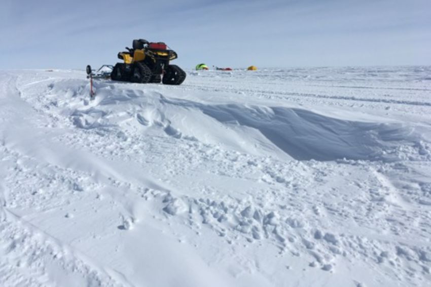
1798                              C. K. Crockart et al.: El Niño–Southern Oscillation signal in a new East Antarctic ice core

pha”, “Bravo”, and “Charlie”, 20–25 m depth). The Main            vestigate the optimal sample resolution over the satellite era
core was drilled from 4 m using the Hans Tausen drill             for accurate dating, we cut 1.5 cm isotope samples in contrast
(Johnsen et al., 2007; Sheldon et al., 2014), while the Al-       to 3 cm chemistry samples over the upper portion of the ice
pha, Bravo, and Charlie ice cores were drilled from the sur-      cores (∼ 20 m). For detailed information on the trace clean
face using the Kovacs drill system, similar to the one used       discrete analysis technique, see Plummer et al. (2012) and
at Law Dome (Vance et al., 2015; Roberts et al., 2015). The       references therein. The oxygen isotopes and ion chemistry
cores were cut to 1 m “bag” lengths in the field and weighed      in the MBS and LD ice cores were analysed according to
to produce a 1 m resolution density profile for each core. No     established methods (Curran and Palmer, 2001; Curran et al.,
other core processing was conducted in the field. The Bravo       2003; Palmer et al., 2001; Plummer et al., 2012). The VG Iso-
core was collected exclusively for persistent organic pollu-      gas SIRA mass spectrometer was used to determine the ratio
tant analysis so it will not be considered hereafter, although    of oxygen isotopes (δ 18 O) in the LD ice core, while the Pi-
high-resolution water stable isotope analyses from this core      carro L2130-i isotopic water analyser was used to determine
were considered for confirmatory purposes during dating the       the water stable isotopes ratios (δ 18 O and δD) in the MBS ice
records presented here. The upper 0.5–0.8 m of the MBS ice        cores. Isotopic values are expressed as per mil (‰) relative to
cores were excluded in this study, as the year horizons for       the Vienna Standard Mean Oceanic Water (VSMOW) stan-
the top year (i.e. most recent year) are difficult to identify,   dard. The Thermo-Fisher/Dionex ICS3000 ion chromato-
and further analysis is required to refine this dating. Based     graph was used to determine the concentrations of trace ion
on the findings of Vance et al. (2016), the MBS Main core         chemistry (anions and cations), including sea salt concentra-
likely spans the past millennium, and deeper ice core trace       tions (chloride, Cl− ; sodium, Na+ ; magnesium, Mg2+ ), cal-
chemical and isotopic analyses are ongoing. However, pre-         cium (Ca2+ ), and sulfate (SO2−4 ), as well as methanesulfonic
cise dating for this study has only been undertaken on the        acid (MSA). Non-sea-salt sulfate (nssSO2−    4 ) was calculated
upper section of the Main core (∼ 20 m) and two of the short      according to the methods in Plummer et al. (2012) and used
cores (i.e. Alpha and Charlie cores). This period includes the    in this study as a dating aid in addition to the usual suite of
satellite era, where satellite and reanalysis datasets are used   seasonal species mentioned above. Parallel sections of the
to investigate the environmental conditions associated with       MBS Main and Charlie cores were sent to the University of
climate signals preserved in the ice cores.                       Copenhagen for impurity determination by continuous flow
   LD (elevation 1370 m, 66.461◦ S, 112.841◦ E) is also a         analysis (Bigler et al., 2011); however, we only consider the
wet-deposition coastal site located on a small coastal ice cap    initial data available from the discrete analyses performed in
in Wilkes Land in East Antarctica (see Fig. 1). The Dome          Australia in this study.
Summit South core drilling location is 4.6 km south of the
LD summit, has prevailing south-easterly winds and mini-
                                                                  2.3   Ice core dating
mal katabatic influence, and preserves strong maritime sig-
nals (McMorrow et al., 2001; Plummer et al., 2012). Previous      Annual depth layers were assigned to the MBS and LD
studies have reported snow accumulation of 0.680 m yr−1 IE        ice cores using seasonally varying species, principally δ 18 O,
(Roberts et al., 2015; van Ommen et al., 2004) and low mean       nssSO2−       +                      2−     −
                                                                         4 , Na , and the ratio of SO4 / Cl , which has been
wind speeds of 8.3 m s−1 (Morgan et al., 1997). The new LD        shown to be an excellent summer marker in the LD ice cores
ice core used in this study, DSS1617, was drilled in summer       (Plummer et al., 2012). Similar to van Ommen and Mor-
2016/2017 and is intended to replace and extend the upper         gan (1996), the summer maxima in δ 18 O around 10 January
portion of the LD record presented in Vance et al. (2013),        are used. The climatology of hydrogen peroxide (H2 O2 ) is
which used four successive short ice cores to cover the pe-       also used in selected sections for the MBS cores as confir-
riod 1990–2009. The new record presented here will extend         matory dating similar to that used for the LD cores (van Om-
to 2016, increasing overlap with the satellite era (and there-    men and Morgan, 1996). Volcanic ash layers (indicated by
fore calibration period) by 7 years (or 19 %) and reducing        nssSO2−4 peaks) linked to the Pinatubo volcanic eruption in
dating errors associated with combining multiple short ice        the Philippines in mid-1991 were used as a reference depth
core composites. Prior to 1990, the LD ice core record used       horizon to cross-check the annual depth layer chronology
in this study is the same as that used in Vance et al. (2013),    (Plummer et al., 2012; see Fig. 2). Each ice core was dated in-
DSS97. The DSS1617 and DSS97 ice core composites were             dividually and independently, without reference to other site
combined using visual analysis of raw data of overlapping         records to ensure independence of the method.
seasonal cycles in 1989/1990 using key dating analytes (see
Sect. 2.3).                                                       2.4   Snow accumulation rates and sea salt concentration
                                                                        analyses
2.2    Isotope and trace ion chemistry analyses
                                                                  The annual depth layers were used in combination with an
Discrete samples for water stable isotope and trace chemistry     empirical density model (in kg m−3 ; see Eq. 1) to determine
samples were cut under trace clean conditions. In order to in-    the annual ice equivalent snow accumulation rates (hereafter

Clim. Past, 17, 1795–1818, 2021                                                     https://doi.org/10.5194/cp-17-1795-2021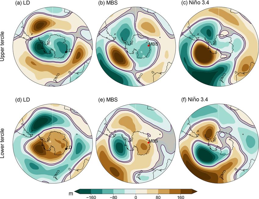
C. K. Crockart et al.: El Niño–Southern Oscillation signal in a new East Antarctic ice core                                     1799

Figure 1. Site map of Mount Brown South (MBS) and Law Dome (LD, Dome Summit South site) in East Antarctica. The embedded table
shows coordinates for the MBS Alpha, Bravo, Charlie, and Main ice core drilling sites.

accumulation) for the MBS ice cores. The empirical den-                polated (i.e. binned) to monthly resolution to determine the
sity model uses the mid-point depth of the annual layer (d             climatology of the sea salts in the MBS and LD records.
in m) and the density of ice (ρ = 917 kg m−3 ), corrects for           Annual rather than seasonal sea salts (and snow accumula-
variations in density in firn, and is based on the methods of          tion) in the MBS ice cores were used for all other analyses
Roberts et al. (2015).                                                 to avoid errors associated with linear interpolation that as-
                                                                       sume uniform accumulation throughout the year. The annual
Empirical Density = [ρ] − [883.5356
                                                                      sea salts in the three MBS ice cores were averaged (here-
                    × exp(−0.011078644 × d)                            after named the site record) to minimize errors associated
                    + [436.8285] − [1.887488 × d]              (1)     with dating uncertainties, such as timing noise (i.e. summer
                                                                       peaking analytes used as dating horizons depend on snow-
Chloride was used as a proxy for sea salt in this study to             fall at the correct time to be preserved accurately, meaning
maintain comparability with Vance et al. (2013), although              that annual averages may include a small portion of signals
sodium was also considered. We acknowledge that Na+ is                 into the adjacent year). McMorrow et al. (2001) suggest that
the more conservative proxy for sea salt (particularly in the          snowfall events at LD have sufficient frequency to preserve
Northern Hemisphere); however, we wished to compare like               monthly signals (i.e. linear interpolation errors are minimal).
for like with LD in Vance et al. (2013). The trace chemistry           In addition, snow accumulation at LD is relatively uniform
analysis in the Australian Antarctic Program Partnership ice           throughout the year, allowing seasonal LD records to be de-
core laboratories is optimized to analyse anions in order to           veloped (Roberts et al., 2015). Previous studies have shown
derive highly accurate methanesulfonic acid (MSA), Cl− ,               that seasonal LD sea salt records preserve signals for climate
SO2−4 , and nitrate (NO3 ) records, meaning that we tend to            modes, such as the ENSO and the Interdecadal Pacific Os-
have fewer gaps in the Cl− record because of this anion pri-           cillation (Vance et al., 2013, 2015); therefore, we consider
ority. Moreover, based on the RACMO estimates of surface               the annual and summer (December–March) concentrations
mass balance (Vance et al., 2016), MBS has sufficient accu-            of sea salt from LD in this study.
mulation (Benassai et al., 2005) to preserve the Cl− record,              To determine variability at the MBS site and between the
similar to LD.                                                         MBS and LD sites, the accumulation and sea salts in the in-
   Sea salt concentrations (Cl− , hereafter sea salts) were            dividual MBS ice cores and the LD record were compared
log-transformed to create a normally distributed record, as            using Pearson’s correlation coefficient. The p values for all
the raw concentrations are skewed toward infrequent high-              analyses in this study are based on effective degrees of free-
concentration events. The sea salts were then linearly inter-

https://doi.org/10.5194/cp-17-1795-2021                                                           Clim. Past, 17, 1795–1818, 2021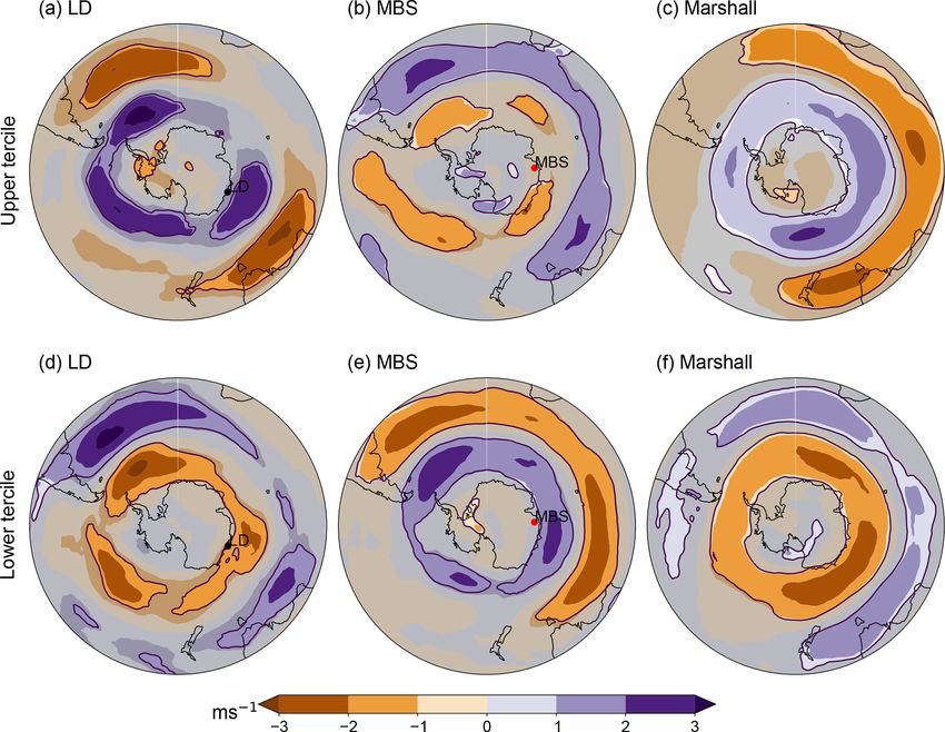
1800                               C. K. Crockart et al.: El Niño–Southern Oscillation signal in a new East Antarctic ice core

Figure 2. An 8 m long section from the Mount Brown South (a MBS1718-Alpha, b MBS1718-Charlie, and c MBS1718-Main) ice cores.
These sections cover the period 1980–1995 (which contains some ambiguous annual horizons; see Sect. 3.1), with annual layers (year
boundaries) shown as triangles with vertical grey lines. Annual horizons are identified from summer-peaking glaciochemical species, i.e.
oxygen isotopes (δ 18 O), non-sea-salt sulfate (nssSO2−                                                 2−   −
                                                     4 ) and the ratio between sulfate and chloride (SO4 / Cl ). Winter-peaking sea salts
   +
(Na ) are used as a confirmatory species. Panels (a) and (b) are on the same depth scale as shown in (c).

Clim. Past, 17, 1795–1818, 2021                                                           https://doi.org/10.5194/cp-17-1795-2021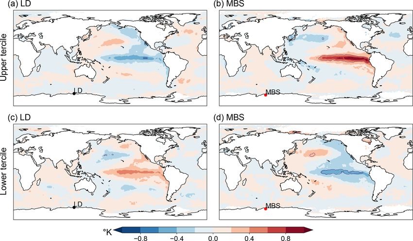
C. K. Crockart et al.: El Niño–Southern Oscillation signal in a new East Antarctic ice core                               1801

dom (Neff ) calculated from a lag-1 autocorrelation, according   the Dipole Mode Index (Saji et al., 1999; available from
to Bretherton et al. (1999). As the dating for the MBS record    http://www.jamstec.go.jp/aplinfo/sintexf/iod/dipole_mode_
is still undergoing incremental improvement and may change       index.html, last access: 3 September 2020). The ENSO,
in the future, analyses of the variability in accumulation and   SAM, and IOD indices were detrended (as were the corre-
sea salts between the ice cores were repeated using a normal-    sponding accumulation and sea salt time series) to reduce
ized Gaussian smooth (kernel = 3 yearly points; σ = 0.6) to      the interference of any climate change signal or long-term
minimize the influence of timing inaccuracies within approx-     trends and ensure any significance was due to interannual
imately 1 year.                                                  variability, rather than (for example) the pronounced shift
                                                                 toward the positive SAM phase during austral summer in
2.5   Instrumental climate data
                                                                 recent decades (Marshall, 2003; Thompson et al., 2000).

To determine whether the MBS site record preserves signals       2.6   Reanalysis and model data
of regional or hemispheric climate variability, the degree of
correlation (lag-0) between the annual accumulation and sea      To investigate atmospheric processes leading to the preser-
salts against seasonal indices for the ENSO, SAM, and IOD        vation of any climate signals, KNMI Climate Explorer (see
was determined using Pearson’s correlation coefficient. Sea-     https://climexp.knmi.nl/start.cgi, last access: 8 April 2021)
sonal indices, rather than annual, were used as these climate    was used to create composite maps of SST, zonal winds, and
modes have their own temporal cycles that do not match           geopotential height anomalies during the upper and lower
the calendar year. For correlation against the annual MBS        terciles of sea salt years in the MBS site and LD records.
record, seasonal SAM indices were derived (i.e. DJF, MAM,        These fields were detrended in order to focus on the inter-
JJA, SON), as the SAM exhibits high-frequency variability        annual variability of the climate modes. The SST anomalies
(weekly to seasonal). The ENSO indices were derived as av-       were constructed using the HadISST observational dataset.
erage June–November SST anomalies, as convection anoma-          The zonal wind and geopotential height anomalies were
lies related to the ENSO tend to emerge in early austral win-    constructed using the ERA5 reanalysis dataset, which has
ter in the equatorial and south-west Pacific and propagate to    an improved grid resolution (0.25◦ × 0.25◦ , ∼ 27 × 10 km
higher southern latitudes during austral spring and into sum-    at MBS) compared to the commonly used ERA-Interim
mer (Fogt and Bromwich, 2006; L’Heureux and Thompson,            (0.75◦ × 0.75◦ , Tetzner et al., 2019). Zonal wind at 500 hPa
2006). In addition, we wished to align as closely as practica-   (instead of surface zonal winds) was chosen to reduce the
ble to the seasonal cycle of sea salt concentrations at MBS,     influence of katabatic winds and topography. The p values
which is likely highest during austral autumn to spring (sim-    used for hypothesis significance testing were computed to in-
ilar to LD) due to decreased mid-latitude storminess in sum-     dicate regions where anomalies are significant at the 90 %
mer (Goodwin et al., 2004; see Fig. A3). We derived an aus-      level. The composite years were based on anomalous sea
tral spring IOD Index to align with the peak of IOD activ-       salt years, while the months displayed were chosen based on
ity (Cai et al., 2013). As the summer LD sea salt record is      months that had significant correlations with the relevant cli-
known to preserve signals for climate modes (Vance et al.,       mate modes.
2013, 2015), the summer record was correlated against sea-          To determine the reliability of the snow accumulation rates
sonal climate indices as defined in Vance et al. (2013), in      derived from the independent layer counting, the accumula-
order to extend their analyses from 2009 to 2016 but remain      tion rates for the MBS ice cores were compared to the an-
comparable with this previous work. Note that we chose to        nual snowfall precipitation from ERA5. The weighted aver-
use a standard spring for the ENSO SST indices (September–       age precipitation from the four neighbouring geographic pix-
November) rather than the September–October average used         els was used to represent accumulation at the MBS ice core
in Vance et al. (2013).                                          site (see Fig. A4). As high wind speeds can remove snow, we
   The ENSO indices used in this study include the               also sought to determine whether snowfall precipitation from
Southern Oscillation Index (Parker, 1983; available              ERA5 would be a useful comparison to ice-core-derived ac-
from       http://www.bom.gov.au/climate/current/soi2.shtml,     cumulation in the first case. Guided by the findings of Li
last access: 3 September 2020), the Multivariate                 and Pomeroy (1997), who determined a dry snow saltation
ENSO Index (Wolter and Timlin, 2011; available from              wind speed threshold of 7.7 m s−1 , we used coincident ERA5
https://psl.noaa.gov/enso/mei/, last access: 3 September         near-surface wind to investigate the presence of a threshold
2020), and the Niño 3.4 and Niño 4 SST indices (Trenberth,       for wind removal of fresh snow. We computed the correla-
1997; available from https://climatedataguide.ucar.edu/          tion between annual total ice core accumulation and annual
climate-data/nino-sst-indices-nino-12-3-34-4-oni-and-tni,        total ERA5 precipitation occurring during times when the
last access: 3 September 2020). The SAM Index used in this       wind speed was lower than a particular threshold. We per-
study is the Marshall Index (Marshall, 2003; available from      formed this sensitivity test for a range of wind speeds from
https://legacy.bas.ac.uk/met/gjma/sam.html, last access:         0 to 30 m s−1 . We also used the surface mass balance output
3 September 2020). The IOD Index used in this study is           from the Modele Atmospherique Region (MAR; Gallee and

https://doi.org/10.5194/cp-17-1795-2021                                                     Clim. Past, 17, 1795–1818, 2021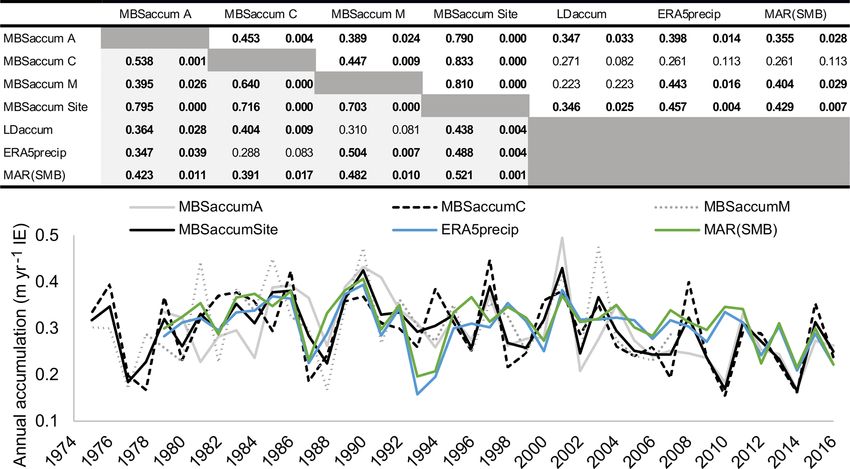
1802                              C. K. Crockart et al.: El Niño–Southern Oscillation signal in a new East Antarctic ice core

Schayes, 1994) to infer the climatology of snow net accumu-        0.295 ± 0.08, and 0.309 ± 0.08 m yr−1 IE, respectively. The
lation. MAR is a regional climate model, specifically devel-       accumulation rates in the three MBS ice cores are signifi-
oped for representing the climate of polar ice sheets, that im-    cantly correlated in all cases, and these correlations increase
proves the representation of the stable boundary layers and        after smoothing (see table insert in Fig. 3). The MBS Al-
feedbacks with snow through sublimation and erosion and            pha and MBS site accumulation records are significantly
deposition processes. We used version 3.11 of MAR, which           correlated with the LD accumulation record (see table in-
has a 35 × 35 km2 horizontal resolution over the Antarctic         sert in Fig. 3). The ERA5 estimate of annual snow accu-
domain and is driven by the ERA5 reanalysis at the bound-          mulation rate for the MBS site record is 0.302 ± 0.05 m yr−1
ary conditions (see Kittel et al., 2021, for more details on the   IE, while the MAR estimate of annual snow accumulation
Antarctic set-up and description of the model version). MAR        is 0.314 ± 0.05 m yr−1 IE. The sensitivity test indicated that
has been thoroughly evaluated against meteorological obser-        the annual precipitation derived from ERA5 correlated most
vations and surface mass balance values over the Antarctic         highly with ice core accumulation when the threshold for
ice sheet (Agosta et al., 2019; Kittel et al., 2021). MAR bet-     wind saltation was set very high (i.e. the net effect of wind
ter reproduces sublimation of precipitation in the katabatic       distribution is close to zero at MBS), and again this indi-
layer over the coastal region (Grazioli et al., 2017), which is    cates the success of the comprehensive study undertaken to
likely underestimated in the atmospheric layers of RACMO           determine the site selection for MBS (Vance et al., 2016).
(Agosta et al., 2019). We preferenced MAR to RACMO, as             The degree of correlation between the accumulation in the
Vance et al. (2016) showed that RACMO (version 2.1/ANT)            MBS ice cores with ERA5 and MAR accumulation estimates
underestimated surface mass balance in the MBS region.             are high and significant, with the exception of Charlie, espe-
We use MAR monthly and 3-hourly surface mass balance               cially when considering the independence of the two tech-
interpolated using a four-nearest inverse-distance-weighted        niques (atmospheric reanalysis-derived site average versus
method at the MBS ice core site.                                   independent layer counting; see table insert in Fig. 3). The
                                                                   ERA5 and MAR accumulation estimates suggest 2 consec-
                                                                   utive years of low accumulation may have occurred in se-
3     Results
                                                                   quence (e.g. 1993 and 1994), which is not demonstrated in
3.1    MBS and LD dating, snow accumulation, and sea
                                                                   the layer-counted data (see Fig. 3). Figure 4 shows that the
       salt concentrations
                                                                   climatology of the ERA5 and MAR accumulation estimates
                                                                   at MBS have a relatively uniform distribution on average,
The standard deviations of δ 18 O for repeated measurements        peaking in austral winter (29 % and 34 % of accumulation
of laboratory reference water samples are less than 0.07 ‰         occurs during this season, respectively), followed by autumn
(for the LD ice core) and 0.05 ‰ (for the MBS ice cores).          (28 % and 28 %), spring (23 % and 27 %), and summer (20 %
The MBS site record has a lower mean sample resolution             and 11 %). Months with extreme precipitation and surface
and accumulation (15 samples per year, 0.296 ± 0.06 m yr−1         mass balance can occur in any season (see Fig. 4). There are
IE, and sample sizes of 3 cm) compared to the LD record (24        6 months over the period 1979–2016 with negative surface
samples per year, 0.747 ± 0.15 m yr−1 IE, and sample sizes         mass balance values. These all occur during summer, includ-
of 5 cm) over the period 1975–2016. The currently analysed         ing January 1979, 1992, 1993 and December 1979, 1991,
section of the Charlie ice core covers the period 1975–2016        and 1994. Of note are the coincident summertime negative
(21.31 m depth), the Alpha core covers 1979–2016 (19.88 m          surface mass balance estimates with the previously identi-
depth), and the Main core covers 1975–2007 (21.21 m depth,         fied and difficult to date low accumulation years of 1993 and
extends back likely 1000 years; however, only the upper            1994.
section has been dated at this stage and is thus considered           The mean annual sea salt concentrations in the Al-
here). The new short LD ice core (that extends the satellite-      pha, Charlie, and Main ice cores and the MBS site
era record) covers the period 1990–2016 (drilled to 28.37 m        record are 1.085 ± 0.32, 1.052 ± 0.38, 1.118 ± 0.36, and
from the snow surface in summer 2017), meaning that it re-         1.090 ± 0.31 µEq L−1 (µEq L−1 : micro-equivalents per litre),
places and extends the four short ice cores used in Vance at       respectively, while the mean annual sea salt concentra-
al. (2013). A peak in nssSO2−
                            4 recorded in the MBS ice cores        tion in the LD record is 3.280 ± 1.32 µEq L−1 . The Na+
aligns with the reference horizon for the Pinatubo eruption,       and Cl− MBS data streams are essentially indistinguishable
which occurred in mid-1991 (Plummer et al., 2012). Figure 2        (r = 0.940, p < 0.000). The annual log-transformed sea salt
shows the MBS cores presented here have reference horizons         concentrations from the three MBS ice cores and the LD
attributed to the Pinatubo eruption in late 1991 (Alpha) and       record are not significantly correlated, although the annual
in 1992 (Charlie and Main). Prior to this volcanic signature       sea salt concentrations in the three MBS ice cores and the
are 4–5 years where the annual horizons are harder to discern      summer sea salt concentrations from the LD record are sig-
(e.g. 1986–1990).                                                  nificantly (and negatively; see table insert in Fig. 5) corre-
   The mean annual snow accumulation rates determined in           lated. The correlations between the MBS ice cores increase
the Alpha, Charlie, and Main ice cores are 0.298 ± 0.07,           after smoothing (see table insert in Fig. 5). The sea salt con-

Clim. Past, 17, 1795–1818, 2021                                                      https://doi.org/10.5194/cp-17-1795-2021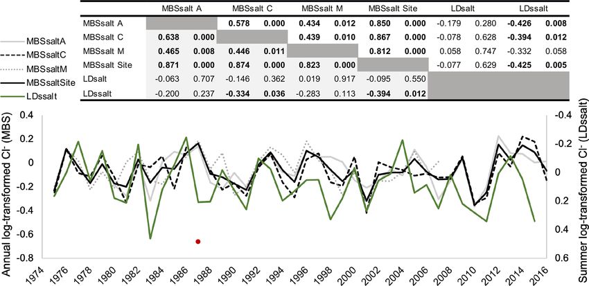
C. K. Crockart et al.: El Niño–Southern Oscillation signal in a new East Antarctic ice core                                        1803

Figure 3. Time series of annual snow accumulation for the Mount Brown South site average (MBSaccumSite); the Alpha (MBSaccumA),
Charlie (MBSaccumC), and Main (MBSaccumM) ice cores; and the ERA5 precipitation data from the MBS Main site (ERA5precip).
The embedded table shows Pearson’s correlation coefficient (r: left column; p: right column) for the average annual snow accumulation for
MBSaccumSite, MBSaccumA, MBSaccumC, and MBSaccumM and the annual snow accumulation for the Law Dome (Dome Summit South
site) record (LDaccum). Correlations using Gaussian-smoothed (kernel = 3 yearly points; σ = 0.6) accumulation time series are shaded and
presented in the lower-left of the table. Correlations significant at 95 % are bold, and the dates range between 1975 and 2016.

Figure 4. Climatology of surface mass balance and precipitation estimates at Mount Brown South from the Modele Atmospherique Regional
(MAR(SMB)) and ERA5 (ERA5precip), respectively, over the period 1975–2016.

centration for the year 1987 in the MBS Charlie ice core               3.2   Climate signals in the MBS and LD ice cores
was excluded from this study (see red dot in time series in
Fig. 5), as it was difficult to discern a year horizon in 1988         The MBS sea salt site record is significantly correlated with
in this core. Further investigation and possible reanalysis of         the seasonal Multivariate ENSO Index, Niño 4, Niño 3.4,
the chemistry data for this year in this core is required before       and the Southern Oscillation Index (June–November; see
including this data in future analyses. The climatology of sea         Table 1). Note that we repeated these correlation analyses
salt at MBS and LD are similar, with a peak in austral winter          using Na+ instead of Cl− for the MBS site record, which
and spring (see Fig. A3).                                              produced virtually identical results (see Table A1). The LD
                                                                       summer sea salt record is also significantly correlated with
                                                                       the seasonal Niño 4, Niño 3.4 (September–November), and

https://doi.org/10.5194/cp-17-1795-2021                                                            Clim. Past, 17, 1795–1818, 2021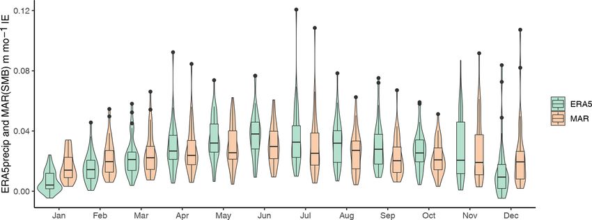
1804                                 C. K. Crockart et al.: El Niño–Southern Oscillation signal in a new East Antarctic ice core

Figure 5. Time series of log-transformed annual sea salt concentrations for the Mount Brown South site average (MBSsaltSite), the Alpha
(MBSsaltA), Charlie (MBSsaltC), and Main (MBSsaltM) ice cores, including the Charlie 1987 (red dot) outlier, and the log-transformed
summer sea salt concentrations for the Law Dome (Dome Summit South site; LDssalt) record (on inverted secondary axis). The embedded
table shows Pearson’s correlation coefficient (r: left column; p: right column) for the log-transformed sea salt concentrations for MBSsaltSite,
MBSsaltA, MBSsaltC, MBSsaltM, LDssalt, and the log-transformed annual sea salt concentrations for the Law Dome (LDsalt) record.
Correlations for normalized Gaussian-smoothed (kernel = 3 yearly points; σ = 0.6) sea salt concentrations are shaded and presented in the
lower-left of the table. Correlations significant at 95 % are bold, and the dates range between 1975 and 2016.

Southern Oscillation Index (November–February; see Ta-                    icant strengthening of the Amundsen Sea Low (note this
ble 1). The MBS–ENSO correlation (positive correlation                    anomaly is shifted toward the west; see Fig. 8e). Compos-
with SST indices) is higher and more significant compared                 ite maps in November–February based on the LD record in-
to the LD–ENSO correlation (negative correlation with SST                 dicate a significant opposite pattern in geopotential height
indices). For example, the highest r value between the an-                anomalies (i.e. strengthening (weakening) of the Amundsen
nual MBS sea salt site record and the June–November ENSO                  Sea Low during the high (low) LD summer sea salt concen-
Index is r = 0.533 and p = 0.001 (Multivariate ENSO In-                   tration years; see Fig. 8a and d). Composite maps based on
dex), whereas the highest r value between the summer LD                   the Niño 3.4 Index (see Fig. 8c and f) show similar geopoten-
sea salt record and the November–February ENSO Index is                   tial height anomalies to those based on the MBS site record,
r = 0.398 and p = 0.01 (Southern Oscillation Index). Fig-                 although they are stronger and more widespread.
ure 6 shows that peaks (troughs) in the MBS sea salt site                    Figure 9 shows composite anomaly maps of the 10 m wind
record generally correspond with peaks (troughs) in the                   in June–August (austral winter) and September–November
Niño 3.4 Index, and the scatter plot therein shows that ex-               (spring) based on high and low sea salt years, along with
treme anomalies (i.e. ENSO events) are reasonably well rep-               maps of the mean 10 m wind. The prevailing wind direc-
resented by the MBS sea salt site record.                                 tion in the MBS region is from the south-east in these sea-
   Composite maps of SST anomalies in June-November                       sons (see Fig. 9a and b). A feature of the winter pattern for
based on high (low) MBS sea salt years indicate significant               the low and high sea salt years (see Fig. 9e and c, respec-
warming (cooling) of the central and eastern equatorial Pa-               tively) is the strong circulation changes north of the MBS
cific (see Fig. 7b and d). Composite maps in November–                    region at around 60◦ S. In winter during low sea salt years
February based on the summer LD sea salts indicate an op-                 (see Fig. 9e), there is a weakening of the prevailing westerly
posite trend in SST anomalies (i.e. warming (cooling) in the              flow associated with general circulation around an anoma-
central and eastern equatorial Pacific during the low (high)              lous cyclonic feature to the north of MBS and an anomalous
LD summer sea salt years); however, these anomalies are not               strengthening of the prevailing easterlies closer to the MBS
significant (see Fig. 7a and c). Composite map of geopoten-               site. In winter during high sea salt years (see Fig. 9c), there
tial height anomalies at 500 hPa in June–November based                   is a strengthening of the prevailing westerly flow around an
on high MBS sea salt years corresponds with a significant                 anomalous anti-cyclonic feature and an anomalous weaken-
weakening of the Amundsen Sea Low (see Fig. 8b), while                    ing of the polar easterlies centred over the ice edge in win-
low sea salt concentration years correspond with a signif-                ter. In spring, the off-shore and on-shore patterns are weaker

Clim. Past, 17, 1795–1818, 2021                                                                https://doi.org/10.5194/cp-17-1795-2021
C. K. Crockart et al.: El Niño–Southern Oscillation signal in a new East Antarctic ice core                                          1805

Table 1. Pearson’s correlation coefficient for the detrended accumulation (MBSaccumSite) and detrended annual log-transformed sea salt
concentrations for the Mount Brown South site average (MBSsaltSite) and the detrended summer log-transformed sea salt concentration
(LDssalt) for the Law Dome (Dome Summit South site) record against detrended seasonal ENSO, SAM, and IOD indices. Correlations
significant at 95 % are bold, and the dates range between 1975–2016.

                                                                      Seasonal indices              Range     r value   p value
          MBSsaltSite        ENSO (Multivariate ENSO Index)           JJASON                   1979–2016      0.533       0.001
                             ENSO (4 Index)                           JJASON                   1975–2016      0.521       0.000
                             ENSO (3.4 Index)                         JJASON                   1975–2016      0.457       0.002
                             ENSO (Southern Oscillation Index)        JJASON                   1975–2016     –0.496       0.001
                             SAM (Marshall Index)                     DJF (January year)       1975–2016      0.107       0.498
                             SAM (Marshall Index)                     MAM                      1975–2016      0.274       0.079
                             SAM (Marshall Index)                     JJA                      1975–2016      0.175       0.266
                             SAM (Marshall Index)                     SON                      1975–2016     −0.168       0.287
                             SAM (Marshall Index)                     DJF (December year)      1975–2016     −0.203       0.196
                             IOD (Dipole Mode Index)                  SON                      1975–2016      0.231       0.140
          LDssalt            ENSO (Multivariate ENSO Index)           SON                      1979–2016     −0.287       0.073
                             ENSO (4 Index)                           SON                      1975–2016     –0.347       0.026
                             ENSO (3.4 Index)                         SON                      1975–2016     –0.332       0.034
                             ENSO (Southern Oscillation Index)        NDJF                     1975–2016      0.398       0.010
                             SAM (Marshall Index)                     DJFM                     1975–2016      0.270       0.087
                             IOD (Dipole Mode Index)                  SON                      1975–2016     −0.122       0.449
          MBSaccumSite       ENSO (Multivariate ENSO Index)           JJASON                   1979–2016      0.226       0.173
                             ENSO (4 Index)                           JJASON                   1975–2016      0.213       0.175
                             ENSO (3.4 Index)                         JJASON                   1975–2016      0.147       0.353
                             ENSO (Southern Oscillation Index)        JJASON                   1975–2016     −0.104       0.511
                             SAM (Marshall Index)                     DJF (January year)       1975–2016      0.150       0.342
                             SAM (Marshall Index)                     MAM                      1975–2016      0.065       0.684
                             SAM (Marshall Index)                     JJA                      1975–2016      0.043       0.787
                             SAM (Marshall Index)                     SON                      1975–2016      0.159       0.313
                             SAM (Marshall Index)                     DJF (December year)      1975–2016     −0.145       0.361
                             IOD (Dipole Mode Index)                  SON                      1975–2016      0.148       0.348

Figure 6. Time series of the annual detrended, log-transformed sea salt concentrations for the Mount Brown South site average (MBSsaltSite)
and the detrended (June–November) El Niño–Southern Oscillation region SST anomalies (ENSO, Niño 3.4 Index). The embedded scatter
plot shows the relationship between the two time series differentiated by positive (red dots) and negative (blue dots) Niño 3.4 region SST
anomalies based on the period 1975–2016.

(see Fig. 9d and f) and their potential influence on frontal            MBS site and LD sea salt records are also not significantly
passages is less clear.                                                 correlated with the spring IOD (Dipole Mode Index) or the
   Table 1 shows that the annual accumulation records from              seasonal MBS and December–March LD SAM (Marshall In-
the MBS site and LD records are not significantly correlated            dex, see Table 1). Despite the lack of a statistically significant
with any of the climate mode indices investigated here. The             SAM signal in the annual MBS sea salt site record, com-

https://doi.org/10.5194/cp-17-1795-2021                                                             Clim. Past, 17, 1795–1818, 2021
1806 C. K. Crockart et al.: El Niño–Southern Oscillation signal in a new East Antarctic ice core Figure 7. SST anomaly composite maps during the upper (a) and lower (c) tercile (November–February) of the detrended, log-transformed summer sea salt concentrations from the Law Dome (LD, Dome Summit South site) record over 1975–2015, and upper (b) and lower (d) tercile (June–November) detrended, log-transformed sea salt concentrations from the annual Mount Brown South (MBS) site average over 1975–2016. The red dot indicates MBS, and the black dot indicates LD. Significant anomalies are within the upper and lower purple contour lines, wherep < 0.1. Figure 8. Geopotential height composite anomaly maps (metres at Z500) during the upper (a) and lower (d) tercile (November–February) of the detrended, log-transformed summer sea salt concentrations from the Law Dome (LD, Dome Summit South site) record over 1979–2015. (b, e) The same as (a) and (d) except using the detrended, log-transformed annual sea salt concentrations from the Mount Brown South (MBS) site average (June–November) over the period 1979–2016. (c, f) The same as (b) and (e) except using the detrended Niño 3.4 Index (June–November). The red dot indicates MBS, and the black dot indicates LD. Significant anomalies are within the upper and lower purple contour lines, where p < 0.1. Clim. Past, 17, 1795–1818, 2021 https://doi.org/10.5194/cp-17-1795-2021
C. K. Crockart et al.: El Niño–Southern Oscillation signal in a new East Antarctic ice core 1807
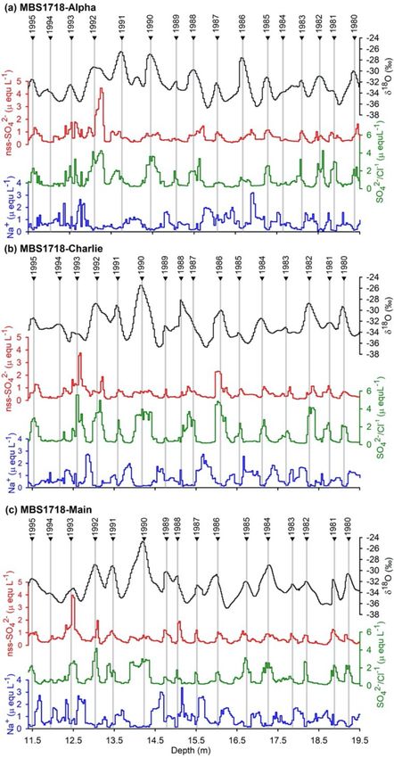
Figure 9. Near-surface (10 m) wind vector composite maps of the mean state during austral winter (a, June–August) and spring (b,
September–November) and anomaly composite maps during the upper (c) and lower (e) tercile in June–August of the detrended, log-
transformed annual sea salt concentrations from the Mount Brown South (MBS) site average, over the period 1979–2016. (d, f) The same
as (c) and (e) except in September–November. The red dot indicates the MBS site location. Latitudinal lines are in increments of 5◦ , and
longitudinal lines are in increments of 15◦ .
posite maps show SAM-like patterns in 500 hPa zonal wind although with a more zonally symmetric pattern in the upper
anomalies during austral summer (see Fig. 10b and e). Com- tercile years.
posite maps in December–February based on low MBS sea
salt years indicate a significant enhancement of zonal wind 4 Discussion
anomalies in the high latitudes and a coincident reduction in
the mid-latitudes (see Fig. 10e). The inverse is true for com- 4.1 MBS and LD ice core features 1975–2016
posite maps based on the high MBS sea salt years, with a
significant reduction of zonal wind anomalies in the high lat- The currently dated recent portion of the MBS site record
itudes and enhancement in the mid-latitudes, although the re- fulfils the requirements stated by Vance et al. (2016) of hav-
duction in high-latitude zonal wind anomalies is not symmet- ing an annual snow accumulation rate of at least 0.200–
rical across the Southern Hemisphere (see Fig. 10b). Com- 0.250 m yr−1 IE and a strong teleconnection with the low
posite maps in November–February based on the LD summer latitudes and mid-latitudes and (based on the initial surface
sea salt years indicate an opposite and significant pattern in accumulation rate analysis presented here) will likely date
zonal wind anomalies (i.e. enhancement (reduction) of zonal back 1000 years at 300 m depth. The mean accumulation rate
wind anomalies in the high- (mid-) latitudes during lower ter- at MBS is identical to the findings of Foster et al. (2006;
cile LD sea salt years (see Fig. 10d), and vice versa for upper 0.297 m yr−1 IE over the period 1984–1999), higher than the
tercile sea salt years (see Fig. 10a). Composite maps based on findings of Smith et al. (2002; 0.255 m yr−1 IE, has a range
the SAM Marshall Index (see Fig. 10c and f) show opposite of 10 years of accumulation over the period 1979–1998),
zonal wind anomalies to those based on the MBS site record, and is higher than estimated in Vance et al. (2016; 0.200–
0.250 m yr−1 IE), suggesting that RACMO (used in Vance et
https://doi.org/10.5194/cp-17-1795-2021 Clim. Past, 17, 1795–1818, 20211808 C. K. Crockart et al.: El Niño–Southern Oscillation signal in a new East Antarctic ice core Figure 10. Zonal wind anomaly composite maps (m s−1 at 500 hPa) during the upper (a) and lower (d) tercile (November–February) of the detrended, log-transformed summer sea salt concentrations from the Law Dome (LD, Dome Summit South site) record over the period 1979–2015. (b, e) The same as (a) and (d) except using the detrended, log-transformed annual sea salt concentrations from the Mount Brown South site average (MBS, December–February) over the period 1979–2016. (c, f) The same as (b) and (e) except using the detrended SAM Marshall Index (December–February). The red dot indicates MBS, and the black dot indicates LD. Significant anomalies are within the upper and lower purple contour lines, where p < 0.1. al., 2016) does in fact underestimate net surface mass balance the periodicity of snowfall events at MBS is determined in in this region. There is some variability in individual accu- greater detail and a longer record is developed. mulation years between the MBS ice cores but not enough The lower accumulation rate in the MBS site record com- to suggest that the relatively large sastrugi and drifts (as high pared to the LD record means that MBS may incur more as 0.5 m, i.e. more than the annual accumulation rate derived dating errors if specific seasonally varying species, such as for MBS) observed at the site in 2017/2018 during drilling water stable isotopes, are not preserved. However, the high are a common feature at the site on interannual timescales r values between the ERA5 and MAR accumulation esti- (see Figs. A1 and A2). The mean accumulation rate in the mates and the snow accumulation time series from indepen- new LD record presented here (0.747 ± 0.15 m yr−1 IE) is dently dated MBS ice cores suggest that the dating is reliable, higher than presented in Morgan et al. (1997; 0.678 m yr−1 ), at least during the period examined here (1975–2016). The Roberts et al. (2015; 0.688 m yr−1 ), and van Ommen and interim dating of the MBS ice cores via independent layer Morgan (2010; 0.688 m yr−1 ); however, these studies focus counting shown in this work has not been corrected with ref- on centennial-scale periods, and in fact a higher accumula- erence to the ERA5 or MAR data. This means we can use the tion rate at LD in recent decades compared to the longer- comparison with ERA5 and MAR to determine how and why term average is supported by the findings of van Ommen and independent layer counting may result in dating errors in the Morgan (2010) and Medley and Thomas (2018). The cli- longer record as it is produced. This is an important first step matology of sea salt concentrations in the MBS site record to understanding how dating errors in the long layer-counted and updated LD record are comparable with the LD record MBS ice core may develop and propagate. In both the MBS presented in Curran et al. (2003) and likely result from in- and LD records we assume the correct date for the Pinatubo creased mid-latitude storminess during winter (Goodwin et reference horizons is likely to be late 1991–1993, as exten- al., 2004). However, the lower sample resolution in the MBS sive examination over multiple overlapping records of the site record and the potential for seasonal variability in snow Pinatubo eruption has been undertaken previously (Plummer accumulation identified in this work mean that the clima- et al., 2012). The difference in Pinatubo reference horizon tology of sea salts should be interpreted with caution until years between the three MBS ice cores indicates the possi- Clim. Past, 17, 1795–1818, 2021 https://doi.org/10.5194/cp-17-1795-2021
You can also read