Changes of Conformation in Albumin with Temperature by Molecular Dynamics Simulations
←
→
Page content transcription
If your browser does not render page correctly, please read the page content below
entropy
Article
Changes of Conformation in Albumin with
Temperature by Molecular Dynamics Simulations
Piotr Weber 1,† , Piotr Bełdowski 2, *,† , Krzysztof Domino 3,† , Damian Ledziński 4,†               and
Adam Gadomski 2,†
 1   Atomic and Optical Physics Division, Department of Atomic, Molecular and Optical Physics, Faculty of
     Applied Physics and Mathematics, Gdańsk University of Technology, ul. G. Narutowicza 11/12,
     80-233 Gdańsk, Poland; piotr.weber@pg.edu.pl
 2   Institute of Mathematics and Physics, UTP University of Science and Technology, Kaliskiego 7,
     85-796 Bydgoszcz, Poland; agad@utp.edu.pl
 3   Institute of Theoretical and Applied Informatics, Polish Academy of Sciences, Bałtycka 5, 44-100 Gliwice,
     Poland; kdomino@iitis.pl
 4   Faculty of Telecommunications, Computer Science and Technology, UTP University of Science and
     Technology, 85-796 Bydgoszcz, Poland; damian.ledzinski@utp.edu.pl
 *   Correspondence: piobel000@utp.edu.pl
 †   These authors contributed equally to this work.

 Received: 16 January 2020; Accepted: 29 March 2020; Published: 1 April 2020

 Abstract: This work presents the analysis of the conformation of albumin in the temperature range
 of 300K–312K, i.e., in the physiological range. Using molecular dynamics simulations, we calculate
 values of the backbone and dihedral angles for this molecule. We analyze the global dynamic
 properties of albumin treated as a chain. In this range of temperature, we study parameters of the
 molecule and the conformational entropy derived from two angles that reflect global dynamics in the
 conformational space. A thorough rationalization, based on the scaling theory, for the subdiffusion
 Flory–De Gennes type exponent of 0.4 unfolds in conjunction with picking up the most appreciable
 fluctuations of the corresponding statistical-test parameter. These fluctuations coincide adequately
 with entropy fluctuations, namely the oscillations out of thermodynamic equilibrium. Using Fisher’s
 test, we investigate the conformational entropy over time and suggest its oscillatory properties in the
 corresponding time domain. Using the Kruscal–Wallis test, we also analyze differences between the
 root mean square displacement of a molecule at various temperatures. Here we show that its values
 in the range of 306K–309K are different than in another temperature. Using the Kullback–Leibler
 theory, we investigate differences between the distribution of the root mean square displacement for
 each temperature and time window.

 Keywords: Flory–De Gennes exponent; conformation of protein; albumin; non-gaussian chain;
 non-isothermal characteristics; Fisher’s test; Kullback–Leibler divergence

1. Introduction
    The dynamics of proteins in solution can be modeled by a complex physical system [1], yielding
many interesting effects such as the competition and cooperation between elasticity and phenomena
caused by swelling. Biopolymers, such as proteins, consist of monomers (amino acids) that are
connected linearly. Thus, a chain seems to be the most natural model of such polymers. However,
depending on the properties of the polymer molecule, modeling it as a chain may give more or less
accurate outcomes [2]. The most straightforward approach to the polymer is the freely jointed chain,
where each monomer moves independently. The excluded volume chain effect, which prevents a
polymer’s segments from overlapping, is one of the reasons why the real polymer chain differs from an

Entropy 2020, 22, 405; doi:10.3390/e22040405                                     www.mdpi.com/journal/entropy
Entropy 2020, 22, 405 2 of 21
ideal chain [3]. The diffusive dynamics of biopolymers are discussed further in [4] and the references
therein, and the subdiffusive dynamics are discussed in [5,6]. For a given combination of polymer and
solvent, the excluded volume varies with the temperature and can be zero at a specific temperature,
named the Flory temperature [7]. In other words, at the Flory temperature, the polymer chain becomes
nearly ideal [8]. However, this parameter is global, and a more detailed description of the dynamics is
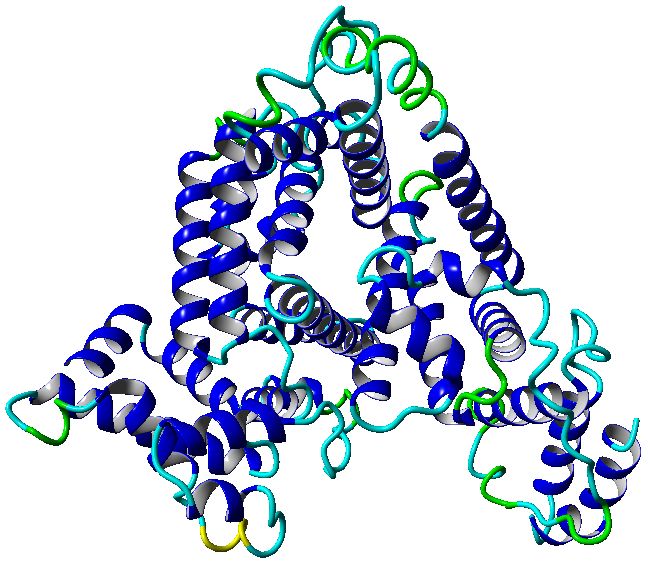
required to perform additional detailed analyses. Our work concentrates on an analysis of albumin
(shown in Figure 1) [9]. Albumin plays several crucial roles as the main blood plasma protein (60%
of all proteins): controlling pH, inducing oncotic pressure, and transporting fluid. This protein (of
nonlinear viscoelastic, with characteristics of rheopexy [10]) plays an essential role in the process of
articular cartilage lubrication [11] by synovial fluid (SF). SF is a complex fluid of crucial relevance for
lowering the coefficients of friction in articulating joints, thus facilitating their lubrication [12]. From a
biological point of view, this fluid is a mixture of water, proteins, lipids, and other biopolymers [13].
As an active component of lubricating mechanisms, albumin is affected by friction-induced increases
of temperature in synovial fluid. The temperature inside the articular cartilage is in the range of
306K–312K [14], and changes occurring inside the fluid can affect the outcome of albumin’s impact
on lubrication [10]. Albumin can help to regulate temperature during fever. Therefore, a similar
mechanism could take place during joint friction, increasing SF lubricating properties as an efficient
heat removal. We analyze this range of temperature: from 300K–312K.
Let us move to the technical introduction of albumin dynamics. Consider a chain that was formed
by N + 1 monomers, assuming the following positions, designated by {~r0 ,~r1 , . . . ,~r N }. We denote
by ~τj = ~r j −~r j−1 a vector of a distance between two neighboring monomers. While considering the
albumin, we have N + 1 = 579 amino acids. For the length of the distance vector ~τj , we take the
distance between two α-carbons in two consecutive amino acids, hence we have |~τj | = τ = 3.8 [Å] [15].
Using such a notation, we can define the end-to-end vector ~R by the following formula:
N
~R = ~r N −~r0 = ∑ ~τj . (1)
j =1
In the case of an ideal chain, the distance vectors (for all Ns) are completely independent of each other.
This property is expressed by a lack of correlation between any two different bonds, that is [16]:
h~τi · ~τj i = τ 2 δij , (2)
where δij is the Kronecker delta. Equations (1) and (2) imply that a dot self-product of vector ~R reads:
N N
h~R · ~Ri = h R2 i = ∑ ∑ h~τi · ~τj i = Nτ2 , (3)
i =1 j =1
where R is the length of the vector ~R. The value of R is measured by calculating the root mean square
end-to-end distance of a polymer. The R’th value is assumed to depend on the polymer’s length N in
the following manner [17]:
R ∼ τN µ , (4)
where µ is called the size exponent. If a chain is freely joined, it appears that µ = 1/2. Relation (4)
suggests we consider the dynamics of the albumin protein in some range of temperature and look for
dependence between the temperature and exponent µ. Applying the natural-logarithm operation to (4)
yields:
log R − log τ
µ' . (5)
log N
In Equation (4) we use a ∼ symbol to emphasize that we use h R2 i to obtain R. In the case discussed
here, both parameters τ and N (the number of amino acids) are constant. Importantly, usingEntropy 2020, 22, 405 3 of 21
molecular dynamics simulations, one can obtain the root mean square end-to-end distance for various
temperatures. The idea of the chain points to its description by backbone angles and dihedral angles.
Backbone angles are angles between three α-carbons occurring after each other and signed by φ. The
second angle, designated by ψ, is a dihedral angle [18]. Using this parametrization, we can obtain an
experimental distribution of probabilities. Such distributions have features that may display some
time-dependent changes.
Figure 1. Structure of the albumin protein in a ribbon-like form. The colors on the molecular surface
indicate the secondary structure: blue—α-helix, green—turn, yellow—3–10 helix, cyan—coil.
These time-dependent changes may have an utterly random course, but sometimes periodic
behavior can be seen. This property can be analyzed using a particular statistical test [19]. There is an
assumption that the time series sampling is even, and the test treats it as a realization of the stochastic
model evolution, which consists of specific terms of the form:
yn = β cos (nω + α) + en , (6)
where β ≥ 0, n = 0, 1, 2, . . . , N, 0 < ω < π, −π < α ≤ π is uniformly distributed in (−π; π ] phase
factor and en is an independent, identically distributed random noise sequence. The null hypothesis is
that amplitude β is equal zero: (H0 : β = 0) against the alternative hypothesis that H1 : β 6= 0.
A periodogram of a time series (y0 , y1 , . . . , y N ) is used to test the above mentioned hypothesis and
it is defined by the following formula:
N 2
1
I (ω ) =
N ∑ exp(−iωj)y j . (7)
j =0
where in general, ω ∈ [0, π ] and i is the imaginary unit. For a discrete time series, a discrete value of ω
from [0, π ] is being used:
2πk
ωk = , k = 0, 1, . . . , N, (8)
N
which are known as Fourier frequencies.Entropy 2020, 22, 405 4 of 21
The periodogram (for a single time series) can contain a peak. The statistical test should give us
information about the significance of this selected peak. It is measured by the p-value parameter. The
statistic which is used in this test has the form:
max1≤i≤q I (ωi )
g= q , (9)
∑ i =1 I ( ωi )
where: I (ωi ) is the spectral estimate (the periodogram) evaluated at Fourier frequencies and q =
[( N − 1)/2] is the entire of the number ( N − 1)/2. The p-value can be calculated according to the
formula [20]:
p
P( g ≥ x ) = ∑ (−1) j−1 nj (1 − jx )n−1 (10)
j =1
where p is the largest integer less than 1/x. In our analysis, we use this framework to evaluate a
p-value for a given time series of entropy. If we get g∗ from the calculation of g, then Equation (10)
gives a p-value for probability that the statistic g is larger than g∗ .
Proteins can be characterized by various parameters that can be obtained from simulations, such
as the earlier mentioned h Ri or µ. Another meaningful parameter is the RMSD (root mean squared
displacement), which can be calculated in every moment of the simulation and is defined as:
r
∑in=1 Ri · Ri
RMSD = (11)
n
where: Ri is a position of the i-th atom. In this way, one can obtain a series of this parameter as a
function of time for the further processing. The drawing procedure is realized at the beginning of the
simulation from the area of initial values. The initial condition for the albumin molecule drawing is
simulated for a given temperature.
We can then group molecules according to mentioned parameters (h Ri, µ, RMSD) and obtain five
sets for 300K, 303K, 306K, 309K, and 312K, and compare these parameters’ values. We decided to use
the Kruscal–Wallis statistical test because it does not assume a normal distribution of the data. This
nonparametric test indicates the statistical significance of differences in the median between sets. A
statistic of this test has the form [21]:
12 k rs2i
H=
N ( N + 1) ∑ ni
− 3( N + 1), (12)
i
where rsi is a sum of all rank of the given sample, N represents the number of all data in all samples,
and k is the number of the groups (set into temperature). We compare the H value of this statistic to the
critical value of the χ2 distribution. If the statistic crosses this critical value, we use a nonparametric
multi-comparison test—the Conover–Iman. The formula which we employ has the form [22]:
s
rsi rs j (Sr − C )( N − 1 − H )
− > t1−α/2 (13)
ni nj ni n j ( N − k )( N − 1)
where Sr is the sum of all square of ranks, t1−α/2 is a quartile from the Student t distribution on N − k
degrees of freedom, and C has the value:
C = 0.25N ( N + 1)2 . (14)
The multi-comparison test gives the possibility of clustering sets of molecules into those between
which there is a statistically significant difference and those between which there is no such difference.
Statistical tests describe differences between medians of the considered sets of molecules.
However, they are not informative about differences between distributions of probabilities. In ourEntropy 2020, 22, 405 5 of 21
work, we use the Kullback–Leibler divergence, which is used in information theory, to compare
two distributions. The Kullback–Leibler divergence between two distributions p and the reference
distribution q is defined as:
pi
KL( p, q) = ∑ pi log . (15)
i
q i
The Kullback–Leibler divergence is also called the relative entropy of p with respect to q.
Divergence defined by (15) is not symmetric measure. Therefore, sometimes one can use a symmetric
form and obtain the symmetric distance measure [23]:
KL( p, q) + KL(q, p)
KLdist ( p, q) = . (16)
2
The measure defined by (15) is called relative entropy. It is widely used, especially for classification
purposes. In our work, we also use this measure to recognize how a given probability distribution is
different from a given reference probability distribution. We can look at this method as a complement
to the Kruscall–Wallis test. The Kruscall–Wallis test gives information about the differences between
medians, while the Kullback–Leibler divergence gives us information about the differences in
distributions.
2. Results
We begin the analysis by examining the global dynamics of molecules at different temperatures
using the Flory theory, briefly described in the introduction. To estimate the exponent µ from definition
in Formula (5), we collect outcomes from a molecular dynamics simulation in the temperature range
of 300K–312K. We use a temperature step of 3K. Such a range of temperature was chosen because we
operated within the physiological range of temperatures. During the simulation, we can follow the
structural properties of molecules in the considered range of temperatures. In the albumin structure,
we can distinguish 22 α-helices, which are presented in Figure 1. Molecules in the given range of
parameters display roughly similar structures. Therefore, we chose to study their dynamics in several
temperatures. One important property, which we can follow during simulations, is a polymer’s
end-to-end distance vector as a function of time. We perform the analysis in two time windows, first,
between 0–30 ns and, second, between 70–100 ns. For each time window, we obtained the root mean
square end-to-end distance of this quantity, whose values are presented in Table 1:
Table 1. Root mean square length of the end-to-end vector for 300K–312K.
Parameter 300K 303K 306K 309K 312K
h R2 i1/2 [Å] for 0 ns–30 ns 47.88 46.69 46.72 47.09 47.81
h R2 i1/2 [Å] for 70 ns–100 ns 47.12 46.67 47.72 47.13 47.64
We can see that the root mean square length of the end-to-end vector for albumin varies with
temperature. To obtain statistics, we can perform the Kruscal–Wallis test of this variation. In our work,
values of the statistics in the test are treated as continuous parameters. We do not specify a statistical
significance threshold. In Table 2, in the second column, we can see the values of statistics calculated
according to Formula (12). The H parameters from the Kruscal–Wallis test have small values for this
test, so the results tend to support the hypothesis about equal medians.Entropy 2020, 22, 405 6 of 21
Table 2. Values of H statistic in the Kruscal–Wallis test for two time windows for a root mean square
end-to-end vector.
Window Value of H
0–30 ns H = 0.62
70–100 ns H = 1.22
The Kruscal–Wallis test only gives information about differences between medians of the sets,
where each set represents one temperature and elements of the set are calculated as root mean square
end-to-end vectors over time. In the analysis, for one temperature, we had the set of root mean
square end-to-end vectors, and in the next step, we calculated a numerical normalized histogram.
Each element of this set corresponds to the single realization of the experiment. The values of the
Kullback–Leibler divergence for mean end-to-end signals in the time window 0–30 ns are presented in
Table 3. In the first column is the reference distribution for the temperature range. We can see that the
biggest value is for the distribution of the temperature 312K in the reference distribution 309K.
Table 3. Kullback–Leibler divergence for root mean square length of mean end-to-end signals in the
time window 0–30 ns. The initial data is the same as for the Kruscal–Wallis test.
Temperature of the Reference Probability 300K 303K 306K 309K 312K
300K 0 0.9324 1.3858 0.8946 0.7604
303K 0.9324 0 1.4628 0.8176 1.6165
306K 0.2802 0.3703 0 0.4096 0.1532
309K 0.9062 0.8161 1.4816 0 2.4139
312K 0.2040 0.3710 0.7023 1.1887 0
We can calculate the Kullback–Leibler distance according to Formula (16). The results are
presented in Table 4. This measure indicates that, between distributions, the biggest differences
are between the distribution for 309K and the distribution for 312K.
Table 4. Symmetric Kullback–Leibler distance for a root mean square length of end-to-end signals in
the time window 0–30 ns. The initial data is the same as for the Kruscal–Wallis test.
300K 303K 306K 309K 312K
300K 0 0.9324 0.8330 0.9004 0.4822
303K 0.9324 0 0.9165 0.8169 0.9938
306K 0.8330 0.9165 0 0.9456 0.4278
309K 0.9004 0.8169 0.9456 0 1.8013
312K 0.4822 0.9938 0.4278 1.8013 0
We can perform the same analyses for the window 70–100 ns. The obtained values of the
Kullback–Leibler divergence, which are presented in Table 5. One can see that the biggest difference is
between the distribution for 312K and the distribution for 303K. One can see that the maximum has
changed and its value is bigger than the maximum for the 0–30 ns window.
Table 5. Kullback–Leibler divergence for a root mean square length of end-to-end signals in the time
window 70–100 ns. The initial data is the same as for the Kruscal–Wallis test.
Temperature of the Reference Probability 300K 303K 306K 309K 312K
300K 0 0.1983 0.1983 0.1409 0.2883
303K 0.7474 0 0.8555 1.6675 2.6390
306K 0.7474 0.8555 0 1.6675 1.1576
309K 0.1351 0.4423 0.4423 0 0.1925
312K 0.8113 1.2084 1.8656 0.7532 0Entropy 2020, 22, 405 7 of 21
For the symmetric case, results are presented in Table 6. We can see that a symmetrical form of
the measure is also between the distribution for 312K and the distribution for 303K.
Table 6. Symmetric Kullback–Leibler distance for a root mean square length of end-to-end signals in
the time window 70–100 ns. The data is the same for the Kruscal–Wallis test.
300K 303K 306K 309K 312K
300K 0 0.4728 0.4728 0.1380 0.5498
303K 0.4728 0 0.8555 1.0549 1.9237
306K 0.4728 0.8555 0 1.0549 1.5116
309K 0.1380 1.0549 1.0549 0 0.4728
312K 0.5498 1.9237 1.5116 0.4728 0
Tables 7–10 give the different statistical approaches, without the averaging over the time step). We
present there all end-to-end signals for one temperature, and for each moment of time, we calculate the
average only over all simulated molecules. In the next step, we calculate normalized histograms. After
obtaining numerical distributions, we calculate the Kullback–Leibler divergence between distributions
of mean end-to-end signals. The results for the time window 0–30 ns are presented in Table 7.
Table 7. Kullback–Leibler divergence between distributions of mean end-to-end signals in the time
window 0–30 ns.
Temperature of the Reference Probability 300K 303K 306K 309K 312K
300K 0 0.1056 0.3194 0.1367 0.1689
303K 0.0939 0 0.2370 0.1261 0.1425
306K 0.2062 0.1450 0 0.1528 0.1841
309K 0.1276 0.1144 0.1877 0 0.2319
312K 0.1288 0.1275 0.2126 0.1848 0
We can see that the large value of the Kullback–Leibler divergence appears for the distribution for
temperature 306K, where the distribution for temperature 300K is a reference distribution. Calculations
for the Kullback–Leibler distance for mean end-to-end signals in the time window 0–30 ns are presented
in Table 8. The results coincide with the measure of Kullback–Leibler divergence.
Table 8. Kullback–Leibler distance for mean end-to-end signals in the time window 0–30 ns.
300K 303K 306K 309K 312K
300K 0 0.0997 0.2628 0.1321 0.1489
303K 0.0997 0 0.1935 0.1202 0.1350
306K 0.2628 0.1935 0 0.1703 0.1984
309K 0.1321 0.1202 0.1703 0 0.2084
312K 0.1489 0.1350 0.1984 0.2084 0
Following the copula approach presented in [24], we performed the bivariate histograms of some
signals to analyse the type of cross-correlation between signals. For the selected example of the mean
end-to-end signals in the 0–30 ns time window see Figure 2, while for the 70–100 ns time window,
see Figure 3. Observe that for the 0–30 ns case, we have simultaneous “high” events, which refer to
the “upper tail dependency”. After the simulation time has passed, this dependency is diminished.
The copula with the “upper tail dependency”, such as the Gumbel one, can provide the proper model
of the mean end-to-end signal for the initial simulation time window. For the later simulation time
window, we should look for the copula with no "tail dependencies", such as the Frank or Gaussian one.Entropy 2020, 22, 405 8 of 21
60
55 101
50
306K
45
40 100
35
40 45 50 55 60 End_to_End__0_30_ns
300K
Figure 2. The bivariate histogram of chosen mean end-to-end signals in the 0–30 ns simulation time
window.
A similar calculation has been performed for the next time window 70–100 ns. In Table 9, we
collect results for Kullback–Leibler divergence for mean end-to-end signals in the time window
70–100 ns.
Table 9. Kullback–Leibler divergence for mean end-to-end signals in the time window 70–100 ns.
Temperature of the Reference Probability 300K 303K 306K 309K 312K
300K 0 0.0920 0.1605 0.1824 0.1183
303K 0.1155 0 0.2969 0.1642 0.1474
306K 0.1108 0.1324 0 0.1621 0.1206
309K 0.1628 0.1266 0.2719 0 0.1206
312K 0.0886 0.0979 0.1356 0.1122 0
Its maximal value is between the distribution for 306K and the distribution for 303K as a reference
distribution.
Table 10. Kullback–Leibler distance for mean end-to-end signals in the time window 70–100 ns.
300K 303K 306K 309K 312K
300K 0 0.1038 0.1356 0.1726 0.1034
303K 0.1038 0 0.2147 0.1454 0.1226
306K 0.1356 0.2147 0 0.2170 0.1281
309K 0.1726 0.1454 0.2170 0 0.1164
312K 0.1034 0.1226 0.1281 0.1164 0
In Table 10 we can see that the biggest value of the Kullback–Leibler distance appears between
the distributions for 306K and 309K. Comparing this result with the previous one, we see that the
maximal Kullback–Leibler distance for the window 0–30 ns changes its place.
In Tables 7–10 the diagonal terms are equal 0, since we comparing a distribution of end-to-end
distributions of raw data for the same time window and temperature. In Table 11 we present selected
Kullback–Leibler distances for distributions of raw data end-to-end signals in the time window
70–100 ns and 306K temperature.Entropy 2020, 22, 405 9 of 21
Table 11. Kullback–Leibler distance for raw data end-to-end signals in the time window 70–100 ns and
306K.
Number of Molecule 1 2 3 4 5 6 7 8 9
1 0 0.2927 0.2073 0.2156 0.2450 0.3016 0.1751 0.2072 0.4298
2 0.2927 0 0.1661 0.0919 0.0931 0.1589 0.2367 0.1310 0.2765
3 0.2073 0.1661 0 0.1347 0.2135 0.3059 0.1282 0.1013 0.1843
4 0.2156 0.0919 0.1347 0 0.1203 0.1353 0.1499 0.1338 0.2585
5 0.2450 0.0931 0.2135 0.1203 0 0.1478 0.2635 0.1434 0.3083
6 0.3016 0.1589 0.3059 0.1353 0.1478 0 0.2812 0.1978 0.3122
7 0.1751 0.2366 0.1282 0.1499 0.2635 0.2812 0 0.1318 0.2281
8 0.2072 0.1310 0.1013 0.1338 0.1434 0.1978 0.1318 0 0.1614
9 0.4298 0.2765 0.1843 0.2585 0.3083 0.3122 0.2281 0.1615 0
60
55
101
50
309K
45
100
40
End_to_End__70_100_ns
40 45 50 55
306K
Figure 3. The bivariate histogram of chosen mean end-to-end signals in the 70–100 ns simulation time
window.
As two different statistical approaches can not unambiguously distinguish between temperatures
(or their subsets), we can conclude that dynamics of the system at this temperatures range is roughly
similar. This will be approved by the analysis of the the Flory–De Gennes exponent.
Using Equation (5), we estimate values of the Flory–De Gennes exponent for the given protein
chain. Results are presented in Table 12. We can see that the values of the Flory–De Gennes exponents
do not differ too much within the examined range of temperature, and they all seem to attain a value
of ca. 0.4. The power-law exponents for oligomers span a narrow range of 0.38–0.41, which is close to
the value of 0.40 obtained for monomers [25–27].
Table 12. Size exponent obtained according to Formula (5).
Parameter 300K 303K 306K 309K 312K
Size exponent (µ) for 0 ns–30 ns 0.3986 0.3947 0.3948 0.3960 0.3984
Size exponent (µ) for 70 ns–100 ns 0.3961 0.3946 0.3981 0.3961 0.3978
Detailed values for two time windows are presented in Table 13. We can see that from a global
point of view and Flory theory, the situation is quite uniform for all initial conditions and is within theEntropy 2020, 22, 405 10 of 21
considered range of temperature. Thus, in our modeling, we see an effect of elasticity vs. swelling.
This competition is preserved for the examined temperature range.
Table 13. Values of H statistic in the Kruscal–Wallis test for µ parameter for two time windows.
Window Value of Parameter H
0–30 ns H = 0.48
70–100 ns H = 1.47
The H parameters from the Kruscal–Wallis test have small values for this test, so the results tend to
support the hypothesis about equal medians.
The distribution of backbone dihedral angles carries information of the molecule’s dynamics, as
they are tightly connected to its elasticity. Using simulations, we can determine the angle φ and the
angle ψ (see Introduction). Next, we can determine energies that depend on these angles by employing
Formula (17). In Figures 4 and 5, we present the logarithm of the angle energy component for two
temperatures. Figure 4 presents values in a period of time 0–10 ns, and Figure 5 presents values in a
period of time 90–100 ns. We can see that these values fluctuate around the mean value. Such dynamics
are similar for all temperatures, but the mean energy rises slightly with increasing temperature. In
Figure 5, the blue line presents a logarithm of the mean value of angle energy and the gray line presents
values of the standard deviation. We can see that changes in energy are much more evident.
T = 300K T = 309K
11.10 ± 11.10 ±
log of angle energy
log of angle energy
11.08 11.08
11.06 11.06
11.04 11.04
11.02 11.02
0 2 4 6 8 10 0 2 4 6 8 10
simulation time [ns] simulation time [ns]
Figure 4. Logarithms of angle energies vs. the simulation time (0–10 ns), exemplary outcome of
T = 300K and T = 309K.
T = 300K T = 309K
11.10 ± 11.10 ±
log of angle energy
log of angle energy
11.08 11.08
11.06 11.06
11.04 11.04
11.02 11.02
90 92 94 96 98 100 90 92 94 96 98 100
simulation time [ns] simulation time [ns]
Figure 5. Logarithms of angle energies vs. the simulation time (90–100 ns), exemplary outcome of
T = 300K and T = 309K.
Different outcomes come from an analysis of the energy component connected with the dihedral
angles ψ. See Figure 6 (blue lines) in double logarithmic scale, and note the linear regression lines. We
present a period of time from 1 ns to 10 ns.Entropy 2020, 22, 405 11 of 21
T = 300K T = 303K T = 306K
11.93 11.93 11.93
log of dihedral energy
log of dihedral energy
log of dihedral energy
11.92 11.92 11.92
11.91 11.91 11.91
4 6 8 10 4 6 8 10 4 6 8 10
log of simulation time [ps] log of simulation time [ps] log of simulation time [ps]
T = 309K T = 312K
11.93 11.93
log of dihedral energy
log of dihedral energy
11.92 11.92
11.91 11.91
4 6 8 10 4 6 8 10
log of simulation time [ps] log of simulation time [ps]
Figure 6. Dihedral energies for each temperature vs. simulation time. We use the double logarithmic
scale. Green lines represent linear regression.
Simulations also show that for further times in the log-log scale, these values exhibit almost no
change with time.
In Figure 7, we present regression parameters from Figure 6.
1e 3 1e 3 1e 3
slope of log dihedral energy vs time
slope of log dihedral energy vs time
slope of log dihedral energy vs time
T = 300K a T = 303K T = 306K
2 a± 2 2
0 0 0
2 2 a 2 a
a± a±
0 20 40 60 0 20 40 60 0 20 40 60
start of 30 long time window [ns] start of 30 long time window [ns] start of 30 long time window [ns]
1e 3 1e 3
slope of log dihedral energy vs time
slope of log dihedral energy vs time
T = 309K T = 312K
2 2
0 0
2 a 2 a
a± a±
0 20 40 60 0 20 40 60
start of 30 long time window [ns] start of 30 long time window [ns]
Figure 7. Slope of dihedral angle from regression.
The dynamics of proteins are governed mainly by non-covalent interactions [28]. Therefore, it
would be useful to study other components of energy, such as the Coulomb component and the van
der Waals component ( see Equation (17) and the discussion following it). The Coulomb component
oscillates around the almost constant trend present for every temperature. However, the mean value
of these oscillations increases with the temperature. The opposite situation appears for the van der
Waals component. Similar to the Coulomb component, for each selected temperature, it follows an
almost constant trend. However, when the temperature increases, the mean value of such oscillations
decreases. The Coulomb component and the van der Waals component obey simple dynamics. Hence,
we can move to a further discussion of more interesting dihedral and angular parts of the energy.Entropy 2020, 22, 405 12 of 21
Simulations of albumin dynamics can be used to obtain frequency distributions of angles φ and
ψ. An exemplary 2 D histogram of such a distribution is presented in Figure 8. We can see that most
data are concentrated in a small area of space of angles. Similar behavior can be observed for other
temperatures and simulation times. This is because the structure of the investigated protein is quite
rigid, and there appears to be only a little angular movement. Nevertheless, we can observe variations
of the conformational entropy, estimated with such a histogram (see Figure 9).
1.6e-03
150
1.4e-03
100
1.2e-03
50 1.0e-03
ψ - angle
0 8.0e-04
−50 6.0e-04
4.0e-04
−100
2.0e-04
−150
0.0e+00
−150 −100 −50 0 50 100 150
φ - angle
Figure 8. Numerically obtained distribution of angles φ and ψ for T = 300K and 30 ns of simulation.
According to formulas connecting the probability distribution of angles and entropy [17], we can
follow changes of entropy in time and temperature. Values of conformational entropy for various
temperatures and with simulation time 0–30 ns are presented in Figure 9, where the blue line represents
the course of the mean entropy value over time. The calculations take into account nine simulations,
and one dot presents one arithmetic mean of entropy. Here, we can see that during simulations, some
oscillations can appear. Therefore, for each temperature, we perform Fisher’s test. Results of this test
are presented in Table 14.
Table 14. Probability (p-value) for mean entropy over time in the time interval 0–30 ns.
300K 303K 306K 309K 312K
p-value 0.849 0.601 0.009 0.536 0.143
A simple comparison of the p-values in Table 14 shows that the lowest value is located around
306K degrees. According to Formula (6), mean entropy is supposed to be treated as stochastic, i.e.,
partially deterministic and partially random. In our work, we treat the p-value as a parameter, which
gives us information about the tendency on maintaining the truth of the hypothesis: β = 0. If the
p-value is lower than in another case, then it presents a stronger tendency in favor of the alternative
hypothesis: β 6= 0.Entropy 2020, 22, 405 13 of 21
T = 300 T = 303 T = 306
41 41 41
a) µ µ±σ b) µ µ±σ c) µ µ±σ
40 40 40
entropy
entropy
entropy
39 39 39
38 38 38
37 37 37
36 36 36
0 10 20 30 0 10 20 30 0 10 20 30
simulation time [ns] simulation time [ns] simulation time [ns]
T = 309 T = 312
41 41
d) µ µ±σ e) µ µ±σ
40 40
entropy
entropy
39 39
38 38
37 37
36 36
0 10 20 30 0 10 20 30
simulation time [ns] simulation time [ns]
Figure 9. Value of conformational entropy for various temperatures and 0–30 ns of simulation time.
Much more detailed calculations of the p-values for this case are presented in Table 15. We can
see that at 306K, there is a local minimum of the mean p-value. It indicates that at 306K, the tendency
towards the alternative hypothesis: β 6= 0 is stronger than it is at 303K and 309K. However, for 300K,
the mean p-value parameter is the smallest. The mean p-value parameter is almost the same for 306K
and 312K. This means that both temperatures exhibit nearly the same tendency for the hypothesis:
β 6= 0. Such regularities can be seen in Figure 9.
Table 15. Probability (p-value) for entropy of single trajectory over time in the time interval 0–30 ns.
Number of Signal 300K 303K 306K 309K 312K
1 0.439 0.737 0.367 0.754 0.643
2 0.153 0.660 0.961 0.922 0.835
3 0.320 0.483 0.012 0.558 0.0551
4 0.263 0.372 0.700 0.223 0.323
5 0.544 0.657 0.057 0.130 0.066
6 0.114 0.385 0.232 0.416 0.360
7 0.499 0.529 0.008 0.006 0.007
8 0.013 0.871 0.610 0.692 0.456
9 0.245 0.891 0.871 0.832 0.694
mean 0.288 0.621 0.424 0.504 0.382
The same analyzes can be done on the data presented in the image.
The same analyzes can be done on the data presented in Figure 10. The results of these analyzes,
in relation to individual time series of entropy, are presented in the Table 16. For these data, we also
observe the local minimum of the p-value parameter for 306K. We have a maximum at 303K. Thus,
the tendency towards the hypothesis β = 0 is strongest here in comparison to the rest of the analyzed
temperatures. This maximum value of the p-value parameter for 303K is also present for the previous
window.Entropy 2020, 22, 405 14 of 21
T = 300 T = 303 T = 306
41 41 41
a) µ µ±σ b) µ µ±σ c) µ µ±σ
40 40 40
entropy
entropy
entropy
39 39 39
38 38 38
37 37 37
36 36 36
70 80 90 100 70 80 90 100 70 80 90 100
simulation time [ns] simulation time [ns] simulation time [ns]
T = 309 T = 312
41 41
d) µ µ±σ e) µ µ±σ
40 40
entropy
entropy
39 39
38 38
37 37
36 36
70 80 90 100 70 80 90 100
simulation time [ns] simulation time [ns]
Figure 10. Value of conformational entropy for various temperatures and 70–100 ns of simulation time.
Table 16. Probability (p-value) for entropy of a single trajectory over time in the time interval 70–100 ns.
Number of Signal 300K 303K 306K 309K 312K
1 0.328 0.720 0.460 0.078 0.041
2 0.183 0.890 0.146 0.713 0.898
3 0.092 0.378 0.219 0.464 0.264
4 0.764 0.800 0.440 0.629 0.297
5 0.030 0.802 0.275 0.323 0.313
6 0.220 0.108 0.330 0.440 0.540
7 0.279 0.121 0.382 0.253 0.046
8 0.582 0.299 0.976 0.324 0.457
9 0.438 0.550 0.438 0.951 0.642
mean 0.324 0.519 0.407 0.464 0.389
Formula (11) can be calculated for each moment of simulation, so we obtain a time series. To get
one parameter for one molecule, we calculate a mean value of this parameter for each molecule. In the
next step, we can perform the same statistical considerations to derive values of the H statistic. For
the time window 0–30 ns, the value of the Kruscal–Wallis test gives H = 9.41; however, for the time
window 70–100 ns, the value of this statistic is H = 12.52. Because we treat the statistic as an ordinary
parameter, we do not specify whether results are significantly different. In our approach, we conclude
that the tendency for the alternative hypothesis about not equal medians is much higher for the time
window 70–100 ns. Since this tendency is more significant in the second case than in the previous one,
we decided to perform a multi-comparison test. We chose the Conover–Iman multi-comparison test.
We treated tα−1/2 as a parameter, which depends on an assumed statistical significance. Therefore in
Table 17, we only give the left side of Equation (13).
Table 17. Results of the Conover–Iman multi-comparison test in the time interval 70–100 ns.
Set of Molecule 300K 303K 306K 309K 312K
300K - 1.2222 16.1111 12.5556 10.3333
303K 1.2222 - 17.3333 13.7778 11.5556
306K 16.1111 17.3333 - 3.5556 5.7778
309K 12.5556 13.7778 3.5556 - 2.2222
312K 10.3333 11.5556 5.7778 2.2222 -
Here, we have a comparison between medians for different sets. Using values from Table 17 and
calculating the right sight of Equation (13) for p = 0.05, we can state that there are sets that differ fromEntropy 2020, 22, 405 15 of 21
another cluster of sets. The cluster of sets for temperatures 306K, 309K, and 312K differ from the set for
temperature 303K. Unfortunately, the set for temperature 300K is between these two.
We can compare the above statistical results to the other methods such as the Kullback–Leibler
distance, which is presented in the Introduction. In Table 18, we have values of this quantity. We
can see that the biggest value is between the distribution for 300K and the distribution for 306K as a
reference distribution.
The calculation of the Kullback–Leibler distance is presented in Table 19. We can conclude that
the 306K case differs most from all other cases, so the dynamics of the system in the temperature range
of 306K–309K appears to differ most from the dynamics of the system in other temperature ranges.
Table 18. Kullback–Leibler divergence for the mean RMSD in the time window 0–30 ns. The data are
the same as for the Kruscal–Wallis test.
Temperature of Reference Distribution 300K 303K 306K 309K 312K
300K 0 0.4045 2.0767 2.917 0.1932
303K 1.6280 0 1.6853 2.4913 0.6891
306K 3.3967 2.6057 0 1.8597 2.3939
309K 2.2053 0.5003 1.1502 0 1.1444
312K 0.1598 0.1343 1.6845 2.5806 0
Table 19. Symmetric Kullback–Leibler distance for the mean RMSD in the time window 0–30 ns. The
data are the same as for the Kruscal–Wallis test.
300K 303K 306K 309K 312K
300K 0 1.0162 2.7367 2.5600 0.1765
303K 1.1016 0 2.1455 1.4958 0.4117
306K 2.7367 2.1455 0 1.5049 2.0392
309K 2.5600 1.4958 1.5049 0 1.8625
312K 0.1765 0.4117 2.0392 1.8625 0
The calculations of Kullback–Leibler divergence and distance for the time window 70–100 ns are
presented in Tables 20 and 21. We can conclude that the biggest value is between the distributions for
306K and 303K.
Table 20. Kullback–Leibler divergence for a mean RMSD in the time window 70–100 ns. The data are
the same as for the Kruscal–Wallis test.
Temperature of Reference Distribution 300K 303K 306K 309K 312K
300K 0 0.2941 2.7930 2.1527 3.9428
303K 0.8374 0 5.1756 2.2304 3.7127
306K 1.3305 2.4804 0 0.8902 2.8295
309K 4.0173 3.3975 3.3421 0 2.7354
312K 3.6680 2.2372 3.3862 0.8271 0
Table 21. Symmetric Kullback–Leibler distance for the mean RMSD in the time window 70–100 ns. The
data are the same as for the Kruscal–Wallis test.
300K 303K 306K 309K 312K
300K 0 0.5657 2.0617 3.0850 3.8054
303K 0.5657 0 3.8280 2.8139 2.9749
306K 2.0617 3.8280 0 2.1161 3.1078
309K 3.0850 2.8139 2.1161 0 1.7812
312K 3.8054 2.9749 3.1078 1.7812 0Entropy 2020, 22, 405 16 of 21
In a further analysis, we compare distributions from signals of the RMSD obtained in the same way
as a mean root square of end-to-end signals. Results for the Kullback–Leibler distance are presented
in Tables 22 and 23. We can conclude that for the time window 0–30 ns, the most significant value
of differences is for the distribution for 309K and the distribution for 300K. For the time window
70–100 ns, the most significant value is for 306K and 303K.
Table 22. Symmetric Kullback–Leibler distance for signals of the RMSD in the time window 0–30 ns.
300K 303K 306K 309K 312K
300K 0 0.3686 0.7090 1.7109 0.1870
303K 0.3686 0 0.3051 1.2909 0.1838
306K 0.7090 0.3051 0 0.7468 0.5706
309K 1.7109 1.2909 0.7468 0 1.4513
312K 0.1870 0.1838 0.5706 1.4513 0
Table 23. Symmetric Kullback–Leibler distance for signals of the RMSD in the time window 70–100 ns.
300K 303K 306K 309K 312K
300K 0 0.1056 6.3487 5.5232 3.9800
303K 0.1056 0 6.4065 5.7737 4.3824
306K 6.3487 6.4065 0 0.9648 1.7829
309K 5.5232 5.7737 0.9648 0 0.4260
312K 3.9800 4.3824 1.7829 0.4260 0
In all tables of the Kullback–Leibler divergence measures we can see 0 value. For all these cases
we compare two raw data from the same time window in the same temperature. Results for 306K we
present in Table 24. We can see that the distribution of Kullback–Leibler distances are widely dispersed.
We can observe a similar dispersion in other temperatures.
Table 24. Symmetric Kullback–Leibler distance for raw signals of the RMSD in the time window
70–100 ns for 306K.
Number of Molecule 1 2 3 4 5 6 7 8 9
1 0 1.669 0.388 0.277 0.137 0.500 3.260 0.560 0.249
2 1.669 0 1.974 2.565 2.074 1.615 0.660 1.498 1.410
3 0.388 1.974 0 0.241 0.617 0.246 3.589 0.299 0.352
4 0.277 2.565 0.241 0 0.250 0.494 3.867 0.628 0.406
5 0.137 2.074 0.617 0.250 0 0.540 3.593 0.597 0.275
6 0.500 1.615 0.246 0.494 0.540 0 3.338 0.080 0.140
7 3.257 0.660 3.589 3.867 3.593 3.337 0 3.118 2.795
8 0.560 1.498 0.300 0.628 0.597 0.080 3.118 0 0.165
9 0.249 1.410 0.352 0.406 0.275 0.140 2.795 0.165 0
Referring to Figure 11, we observe simultaneous small valued events for the 0–30 ns simulation
time window. There is no such events for the 70–100 ns simulation time window, see Figure 12. Here,
the copula with the “lower tail dependency”, such as the Clayton, can provide the proper model of the
RMSD for the 0–30 ns simulation time window.Entropy 2020, 22, 405 17 of 21
3.0
2.5
2.0
101
309K
1.5
100
1.0
0.5 RMSD1__0_30_ns
0.5 1.0 1.5 2.0 2.5
300K
Figure 11. The bivariate histogram of the chosen mean RMSD signals in the 0–30 ns simulation time
window.
3.30
3.25
101
3.20
3.15
306K
3.10
3.05 100
3.00
RMSD1__70_100_ns
2.6 2.7 2.8 2.9
303K
Figure 12. The bivariate histogram of the chosen mean RMSD signals in the 70–100 ns time window.
3. Discussion
Albumin plays an essential role in many biological processes, such as the lubrication of articular
cartilage. Hence, knowledge of its dynamics in various physiological conditions can help us to
understand better its role in reducing friction. From a general point of view, albumin behaves stable
regardless of the temperature. The angle energy of the protein fluctuates similarly regardless of the
temperature (see Figures 4 and 5). However, its mean value rises monotonically with temperature. On
the other hand, the size exponent µ fluctuates with temperature. We calculate, using the Kruscal–Wallis
test, that these fluctuations generate small values of H parameter and, as a result, indicate a hypothesis
about the equality of medians.Entropy 2020, 22, 405 18 of 21
Further, referring to Figures 6 and 7, we can see that the dihedral energy seems to obey (at least
at some range of simulation times) the power law-like relation, although the scaling exponent is
relatively small. In Figure 7, we can see this relation in the range of temperature from 306K–309K.
This exponent does not change in time t too much. It suggests stable behavior. We consider the
conformational entropy of the system. For its plot versus simulation time see Figures 9 and 10. On
each graph, we can observe a pattern which seems to attain an oscillatory behavior. Fisher’s test allows
describing this property by providing the p-value parameter. If this parameter, for some time series of
entropy, is relatively small in contrast to p-value parameters for another time series of entropy, then
the statistical hypothesis H0 :β = 0 is less probable than in another case. In Table 14, we can observe
that in the range of temperature 303K–309K, there is a local minimum of p-values. A similar effect can
be observed in Table 15 when we calculate the mean p-value for each column. We can also observe
that there is a local minimum of around 306K. A smaller mean p-value is seen for 300K and 312K. This
means that both temperatures exhibit the analogical tendency to favor the hypothesis β 6= 0. We can
also see this in Figure 9, where for temperatures 300K, 306K, and 312K, the regularity of periodicity
increases more than at other temperatures. Other tests, including the Kruscal–Wallis test followed by
the Conover–Iman multi-comparison test, Kullback–Leibler distance, and Kullback–Leibler divergence
give consistent results, while referring to the mean RMSD of the protein of interesting.
This globular protein is soluble in water and can bind both cations and anions. By analyzing
Figures 1 and 8, it is clear that albumin’s secondary structure is mainly standard α-helix. Charged
amino acids (AA) have a large share in albumin’s structure, especially Aspartic and Glutamic acid (25%
of all AA) and hydrophobic Leucine and Isoleucine (16%). This composition enables it to preserve
its conformation, due to intramolecular interactions as well as interactions with the solvent. Two
main factors are at play here, namely hydrophobic contacts and hydrogen bonds (which also occur
between protein and water). A large number of charged AA result in a considerable number of inter-
and intramolecular hydrogen bonds. On the other hand, hydrophobic AA result in a more substantial
impact when the hydrophobic effect stabilizes a protein’s core. As shown by Rezaei-Tavirani et al. [29],
the increase of temperature in the physiological range of temperatures results in conformational
changes in albumin, which cause more positively charged molecules to be exposed. This, in turn,
results in a lower concentration of cations near a molecule. Albumin is known to largely contribute to
the osmotic pressure of plasma, where the presence of ions largely influences this property. An increase
of temperature results in a reduction of the osmotic pressure of blood, which in feverish conditions
can lead to a higher concentration of urine. Because water is the main component of blood and it
has a high heat capacity, the increase of urine concentration results in better removal of heat from the
body [29]. The difference in dynamics between temperatures shown in the present study could indicate
albumin’s binding affinity with other SF components and thus changes its role in biolubrication toward
anti-inflamatory. However, due to the high complexity of the fluid, more research has to be performed.
These chemical properties result in an effect of elasticity vs. swelling competition for albumin
chains immersed in water. If the elasticity of the chain fully dominates over albumin’s swelling-induced
counterpart (interactions of polymer beads and water with network/bond creation), the exponent
would have a value of 1/2. If, in turn, a reverse effect applied, the value of the exponent should
approach the value of 1/4, [30] (note the two first Eqs only). As a consequence, and what has not
been discovered by any other study, the exponent obtained from the simulation in the examined range
of temperature looks as if it is near an arithmetic mean of the two exponents mentioned, namely:
µ = 1/2(2/4 + 1/4) = 3/8, thus pointing to 0.375 ∼ 0.4. The difference of about 0.025 very likely
comes from the fact that the elastic effect on albumin shows up to win over the swelling-assisted
counterterm(s), cf. the Hamiltonian used for the simulations. The exponent µ = 3/8 is for itself
called the De Gennes exponent, and it is reminiscent of the De Gennes dimension-dependent gelation
exponent 2/(d + 2), see [30] (eq 15 therein; d = 3-case). It suggests that albumin’s elastic effect,
centering at about 0.4, is fairly well supported by the internal network and thus supports the
creation of bonds, which has been revealed by the present study. Of course, the overall frameworkEntropy 2020, 22, 405 19 of 21
is well-substantiated in terms of the scaling concept [3,7]. Regular oscillations of entropy suggest
that the system oscillates around the equilibrium state. Furthermore, the Flory–De Gennes exponent
appears to be unchanged for both observation windows. Therefore, we expect the system to be near
the equilibrium state. We expect the dynamic of the system, for longer simulation times, to be similar
to the presented one. The AMBER force field has been reported on overstabilizing helices in proteins.
Therefore our next work will report on the effect of force field and water model used.
4. Materials and Methods
The structure of human albumin serum (code 1e78) has been downloaded from a protein data
bank (https://www.rcsb.org/structure/1E78) as a starting point to simulations. We use the YASARA
Structure Software (Vienna, Austria) [31] to perform MD simulations. Besides this, a three-site model
(TIP3P) of water was used [32]. All-atom simulations were performed under the following conditions:
temperature 310K, pH = 7.0 and in 0.9% NaCl aqueous solution, with a time step of 2 f s. Berendsen
barostat and thermostat with a relaxation time of 1 f s were used to maintain constant temperature
and pressure. To minimize the inuence of rescaling, YASARA does not use the strongly fluctuating
instantaneous microscopic temperature to rescale velocities at each simulation step (classic Berendsen
thermostat). Instead, the scaling factor is calculated according to Berendsen’s formula from the time
average temperature. The charge was –15. Simulations were carried for 100 ns, due to the fact that
throughout this time very small fluctuations of entropy measured could be seen. All-atom molecular
dynamics simulations were performed using the AMBER03 force field [33]. The AMBER03 potential
function describing interactions among particles takes into account electrostatic, van der Waals, bond,
bond angle, and dihedral terms:
∑ ∑
2 2
Etotal = k b r − req + k φ φ − φeq
bonds angle
" #
Vn Aij Bij qi q j
+ ∑ [1 + cos (nψ − γ)] + ∑ 12 − 6 + (17)
dihedrals
2 i < j rij rij erij
where, k b and k φ are the force constants for the bond and bond angles, respectively; r and φ are bond
length and bond angle; req and φeq are the equilibrium bond length and bond angle; ψ is the dihedral
angle and Vn is the corresponding force constant; the phase angle γ takes values of either 0◦ or 180◦ .
The non-bonded part of the potential is represented by van der Waals (Aij ) and London dispersion
terms (Bij ) and interactions between partial atomic charges (qi and q j ). e is the dielectric constant.
For each spherical angle distribution, we performed a normalized histogram consisting of 50 bins.
Such a bin number is a compromise between a resolution and smoothness of histograms. Taking the
empirical probability pi of data being in i-th bin, we estimate the entropy [18,34]:
S = − R0 ∑ pi log( pi ), (18)
i
J
where we use the gas constant R0 = 8.314 K ·mol . The sum goes over the discretized Ramachandran
space. Obviously, since entropy is an information measure, it depends on a bin size, hence we have
here only an estimation applicable for entropy comparisons for different temperatures and simulation
times, since bin sizes are constant for all simulations and temperatures. Numerical data analyzes were
performed in the Scilab development environment [35].
5. Conclusions
We present several scenarios of an analysis of simulations of the albumin dynamics. The albumin
is the linear protein, which makes simulations and analysis straightforward. In particular, we getEntropy 2020, 22, 405 20 of 21
the end-to-end vector values, and we present that changes for exponent do not vary significantly.
The more detailed analysis can be performed, however, using the entropy that appears to oscillate in
the function of the simulation time. In general, these oscillations are regular, which is approved by
employing the statistical test.
However, our findings show that near the 306K temperature, we can observe a local minimum of
the p-value of this test. Interestingly, this minimum changes its position near the 312K temperature for
the 70–100 ns time window. We also consider the RMSD parameter, which for the second time window,
exhibits significant differences between the median of the sets defined for temperatures—we observe
clustering.
When summarizing, let us note that the elastic energy terms included in the Hamiltonian
(Equation (17)) provide a particularly robust bond vs. angle contribution to the elastic energy of the
biopolymer, especially when arguing its role in the angles’ domain. The remaining non-elastic terms
in Equation (17), in turn, contribute, in general, to the swelling assisted co-effect. Thus, the already
mentioned Van der Waals and electrostatic terms are responsible for the overall attraction–repulsion
behavior of the network-like swollen albumin, whereas the last “liquid–crystalline” type of energetic
inclusion to Equation (13) samples the dihedral angles space, an observation already discussed above.
Author Contributions: Conceptualization, P.W., P.B., K.D., and A.G.; investigation, P.W., P.B., K.D., and D.L.;
writing—original draft preparation, P.W. and P.B.; writing—review and editing, P.B., K.D., D.L. and A.G. All
authors have read and agreed to the published version of the manuscript.
Funding: This work is supported by UTP University of Science and Technology, Poland, grant BN-10/19 (P.B.
and A.G.).
Acknowledgments: We wish to thank Maryellen Zbrozek, E.T.A. at UTP (Fulbright fellowship) for her kind help
in assessing the final form of our paper.
Conflicts of Interest: The authors declare no conflict of interest.
References
1. Grimaldo, M.; Roosen-Runge, F.; Zhang, F.; Schreiber, F.; Seydel, T. Dynamics of proteins in solution. Quarter.
Rev. Biophys. 2019, 52, e7.
2. Rubinstein, M.; Colby, R.H. Polymer Physics; Oxford University Press: Oxford, UK, 2003.
3. De Gennes, P.G. Scaling Concepts in Polymer Physics; Cornell University Press: Ithaca, NY, USA, 1979.
4. Gadomski, A. On (sub) mesoscopic scale peculiarities of diffusion driven growth in an active matter confined
space, and related (bio) material realizations. Biosystems 2019, 176, 56–58.
5. Metzler, R.; Jeon, J.H.; Cherstvy, A.G.; Barkai, E. Anomalous diffusion models and their properties:
Non-stationarity, non-ergodicity, and ageing at the centenary of single particle tracking. Phys. Chem.
Chem. Phys. 2014, 16, 24128.
6. Weber, P.; Bełdowski, P.; Bier, M.; Gadomski, A. Entropy Production Associated with Aggregation into
Granules in a Subdiffusive Environment. Entropy 2018, 20, 651.
7. Flory, P. Principles of Polymer Chemistry; Cornell University Press: Ithaca, NY, USA, 1953.
8. Doi, M.; Edwards, S.F. The Theory of The Polymer Dynamics. In The International Series of Monographs on
Physics; Oxford University Press: New York, NY, USA, 1986; pp. 24–32.
9. Bhattacharya, A.A.; Curry, S.; Franks, N.P. Binding of the General Anesthetics Propofol and Halothane to
Human Serum Albumin. J. Biol. Chem. 2000, 275, 38731–38738.
10. Oates, K.M.N.; Krause, W.E.; Jones, R.L.; Colby, R.H. Rheopexy of synovial fluid and protein aggregation. J.
R. Soc. Interface 2006, 3, 167–174.
11. Rebenda, D.; Čípek, P.; Nečas, D.; Vrbka, M.; Hartl, M. Effect of hyaluronic acid on friction of articular
cartilage. Eng. Mech. 2018, 24, 709–712.
12. Seror, J.; Zhu, L.; Goldberg, R.; Day, A.J.; Klein, J. Supramolecular synergy in the boundary lubrication of
synovial joints. Nat. Commun. 2015, 6, 6497, doi:10.1038/ncomms7497.
13. Katta, J.; Jin, Z.; Ingham, E.; Fisher, J. Biotribology of articular cartilage—A review of the recent advances.
Med. Eng. Phys. 2000, 30, 1349–1363.Entropy 2020, 22, 405 21 of 21
14. Moghadam, M.N.; Abdel-Sayed, P.; Camine, V.M.; Pioletti, D.P. Impact of synovial fluid flow on temperature
regulation in knee cartilage. J. Biomech. 2015, 48, 370–374.
15. Liwo, A.; Ołdziej, S.; Kaźmierkiewicz, R.; Groth, M.; Czaplewski, C. Design of a knowledge-based force field
for off-latice simulations of protein structure. Acta Biochim. Pol. 1997 44, 527–548.
16. Havlin, S.; Ben-Avraham, D. Diffusion in disordered media. Adv. Phys. 2002, 51, 187–292.
17. Bhattacharjee, S.M.; Giacometti, A.; Maritan, A. Flory theory for polymers. J. Phys. Condens. Matter 2013, 25,
503101.
18. Baxa, M.C.; Haddadian, E.J.; Jumper, J.M.; Freed, K.F.; Sosnick, T.R. Loss of conformational entropy in
protein folding calculated using realistic ensembles and its implications for NMR-based calculations. Proc.
Natl. Acad. Sci. USA 2014 111, 15396–15401.
19. Ahdesmaki, M.; Lahdesmaki, H.; Yli-Harja, O. Robust Fisher’s test for periodicity detection in noisy
biological time series. In Proceedings of the IEEE International Workshop on Genomic Signal Processing and
Statistics, Tuusula, Finland, 10–12 June 2007.
20. Wichert, S.; Fokianos, K.; Strimmer, K. Identifying periodically expressed transcripts in microarray time
series data. Bioinformatics 2004, 20, 5–20.
21. Kanji, G.K. 100 Statiatical Tests; SAGE Publications Ltd.: Thousand Oaks, CA, USA, 2006.
22. Conover, W.J. Practical Nonparametric Statistics, 2nd ed.; John Wiley & Sons: New York, NY, USA, 1980.
23. Gupta, A.; Parameswaran, S.; Lee, C.-H. Classification of electroencephalography signals for different
mental activities using Kullback-Leibler divergence. In Proceedings of the IEEE International Conference on
Acoustics, Speech and Signal Processing, Taipei, Taiwan, 19–24 April 2009.
24. Domino, K.; Błachowicz, T.; Ciupak, M. The use of copula functions for predictive analysis of correlations
between extreme storm tides. Physica A 2014, 413, 489–497.
25. Tanner, J.J. Empirical power laws for the radii of gyration of protein oligomers. Acta Crystallogr. D Struct.
Biol. 2016, 72, 1119–1129.
26. Korasick, D.A.; Tanner, J.J. Determination of protein oligomeric structure from small-angle X-ray scattering.
Protein Sci. 2018, 27, 814–824.
27. De Bruyn, P.; Hadži, S.; Vandervelde, A.; Konijnenberg, A.; Prolič-Kalinšek, M.; Sterckx, Y.G.J.; Sobott, F.;
Lah, J.; Van Melderen L.; Loris, R. Thermodynamic Stability of the Transcription Regulator PaaR2 from
Escherichia coli O157:H7. Biophys. J. 2019, 116, 1420–1431.
28. Durell, S.R.; Ben-Naim, A. Hydrophobic-Hydrophilic Forces in Protein Folding. Biopolymers 2017, 107,
e23020.
29. Rezaei-Tavirani, M.; Moghaddamnia, S.H.; Ranjbar, B.; Amani, M.; Marashi, S.A. Conformational Study of
Human Serum Albumin in Pre-denaturation Temperatures by Differential Scanning Calorimetry, Circular
Dichroism and UV Spectroscopy. J. Biochem. Mol. Biol. 2006 39, 530–536.
30. Isaacson, J.; Lubensky, T.C. Flory exponents for generalized polymer problems. J. Phys. Lett. 1980, 41,
L-469–L-471.
31. Krieger, E.; Vriend, G. New ways to boost molecular dynamics simulations. J. Comput. Chem. 2015, 36,
996–1007.
32. Mark, P.; Nilsson, L. Structure and Dynamics of the TIP3P, SPC, and SPC/E Water Models at 298 K. J. Phys.
Chem. A 2001, 105, 9954–9960.
33. Duan, Y.; Wu, C.; Chowdhury, S.; Lee, M.C.; Xiong, G.; Zhang, W.; Yang, R.; Cieplak, P.; Luo, R.; Lee, T.; et al.
A point-charge force field for molecular mechanics simulations of proteins based on condensed-phase
quantum mechanical calculations. J. Comput. Chem. 2003, 24, 1999–2012.
34. Baruah, A.; Rani, P.; Biswas, P. Conformational Entropy of Intrinsically Disordered Proteins from Amino
Acid Triads. Sci. Rep. 2015, 5, 11740.
35. SciLab. Available online: https://www.scilab.org (accessed on 30 April 2017).
c 2020 by the authors. Licensee MDPI, Basel, Switzerland. This article is an open access
article distributed under the terms and conditions of the Creative Commons Attribution
(CC BY) license (http://creativecommons.org/licenses/by/4.0/).You can also read