Causal inference and machine learning approaches for evaluation of the health impacts of large-scale air quality regulations
←
→
Page content transcription
If your browser does not render page correctly, please read the page content below
Causal inference and machine learning approaches for evaluation of
                                                the health impacts of large-scale air quality regulations
                                                       Rachel C. Nethery1 , Fabrizia Mealli2 , Jason D. Sacks3 , Francesca Dominici1
                                                        1
                                                            Department of Biostatistics, Harvard T.H. Chan School of Public Health, Boston, MA USA
                                                   2
                                                       Department of Statistics, Computer Science, Applications, University of Florence, Florence, Italy
                                                              3
                                                                  National Center for Environmental Assessment, Office of Research and Development,
arXiv:1909.09611v1 [stat.AP] 15 Sep 2019

                                                                      U.S. Environmental Protection Agency, Research Triangle Park, NC, USA

                                                                                                     Abstract
                                                     We develop a causal inference approach to estimate the number of adverse health events prevented
                                                 by large-scale air quality regulations via changes in exposure to multiple pollutants. This approach is
                                                 motivated by regulations that impact pollution levels in all areas within their purview. We introduce
                                                 a causal estimand called the Total Events Avoided (TEA) by the regulation, defined as the difference
                                                 in the expected number of health events under the no-regulation pollution exposures and the observed
                                                 number of health events under the with-regulation pollution exposures. We propose a matching method
                                                 and a machine learning method that leverage high-resolution, population-level pollution and health data
                                                 to estimate the TEA. Our approach improves upon traditional methods for regulation health impact
                                                 analyses by clarifying the causal identifying assumptions, utilizing population-level data, minimizing
                                                 parametric assumptions, and considering the impacts of multiple pollutants simultaneously. To reduce
                                                 model-dependence, the TEA estimate captures health impacts only for units in the data whose anticipated
                                                 no-regulation features are within the support of the observed with-regulation data, thereby providing a
                                                 conservative but data-driven assessment to complement traditional parametric approaches. We apply
                                                 these methods to investigate the health impacts of the 1990 Clean Air Act Amendments in the US
                                                 Medicare population.
                                                 Keywords: Matching, Bayesian Additive Regression Trees, Counterfactual Pollution Exposures, 1990
                                                 Clean Air Act Amendments

                                           1    Introduction
                                           In its 2011 cost-benefit analysis of the 1990 Clean Air Act Amendments (CAAA), the United States Envi-
                                           ronmental Protection Agency (EPA) estimates that the total direct costs of compliance in the year 2000 were
                                           nearly $20 billion, and it anticipates that these costs will increase to over $65 billion by 2020 (US EPA, 2011).
                                           The CAAA is an expansion of the 1970 Clean Air Act, and it has prompted the enactment of numerous new
                                           regulatory programs, both at national and local levels, to ensure that pollution emissions limits are observed
                                           and that air quality standards are being met (see Henneman et al. (2019) for a summary). Hereafter, for
                                           simplicity we use the term CAAA to refer to the set of regulations put in place to adhere to the law. While
                                           the EPA estimates that the economic benefits of the CAAA dwarf the costs (estimated 2000 benefits $770
                                           billion, estimated 2020 benefits $2 trillion), the increasing compliance costs call for continued evaluations of
                                           the effects of the CAAA using the most advanced, rigorous methods. Of particular interest to the public are
                                           the health impacts of the CAAA.
                                               Traditionally, assessments of the health impacts of large-scale regulations, including assessments of the
                                           CAAA, have relied on the combination of simulated air quality models and pollutant-health exposure-
                                           response functions (ERF). These assessments have relied on various tools including the World Health Orga-
                                           nization’s AirQ+ software (WHO, 2019) and EPA’s Environmental Benefits Mapping and Analysis Program
                                           - Community Edition (BenMAP-CE) software (US EPA, 2011; Sacks et al., 2018). For example, within

                                                                                                         1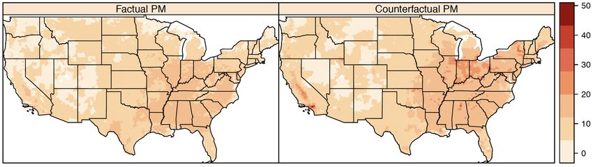
BenMAP-CE, atmospheric chemistry modeling is first used to estimate concentrations of a pollutant on a
grid across the area of interest in a post-regulation year under (1) the factual/observed scenario of regulation
implementation and (2) the counterfactual/unobserved scenario of no regulation (hereafter referred to as
factual and counterfactual exposures). The difference in the factual and counterfactual pollutant levels in
each grid cell are used as inputs in the ERFs. The ERFs employ these differences along with the size of the
exposed population and a health effect estimate, i.e. a linear model coefficient from a previously published
epidemiologic study capturing the relationship between pollutant exposure and a health outcome, to estimate
the number of health events prevented by the regulation-attributable changes in pollutant exposures in the
specified year. This process is performed separately for each relevant pollutant-health outcome combination.
For more detail on the traditional approach and the ERFs, see Section 1 of the Supplementary Materials.
    Causal inference principles have historically been featured heavily in analyses of the health effects of short-
term air pollution interventions, which can often be formulated as natural experiments. Larger, gradually-
implemented regulatory actions are more complex because 1) the resultant changes in levels of multiple
pollutants vary in space and time, 2) long term health trends may coincide with changes in air quality, and
3) time-varying confounding is likely (van Erp et al., 2008). Only recently have causal inference approaches
begun to be developed to address these issues. Zigler et al. (2012) and Zigler et al. (2018) investigate the effect
of a component of the CAAA, the National Ambient Air Quality Standard (NAAQS) non-attainment desig-
nations, on health in the Medicare population using a principal stratification approach. To our knowledge,
factual and counterfactual exposures from air quality modelling software and causal inference methodology
have not yet been integrated for regulation evaluation, despite their natural connection.
    In this paper, we seek to estimate the number of health events prevented by the CAAA in a specific
year using a unique approach that combines factual and counterfactual pollution exposures with observed
health outcome data from the Medicare population (instead of relying on ERFs derived from previously
conducted epidemiologic studies). In particular, we intend to answer the question “How many mortality
events, cardiovascular hospitalizations, and dementia-related hospitalizations were prevented in the Medicare
population in the year 2000 due to CAAA-attributable changes in particulate matter (PM2.5 ) and ozone (O3 )
exposures in the same year?” Because pollution exposures may continue to impact health beyond the year of
exposure, we also wish to determine how many of each of these health events were prevented in the year 2001
due to the CAAA-attributable changes in pollutant exposures in the year 2000. To investigate this question,
we utilize estimates of PM2.5 and O3 exposure levels across the US for the year 2000 under the factual
with-CAAA scenario and under the counterfactual no-CAAA scenario. We combine them with zipcode level
counts of mortality, cardiovascular hospitalizations, and dementia-related hospitalizations from Medicare in
the years 2000 and 2001. Then we utilize the number of health events observed under factual PM2.5 and O3
levels to inform estimation of the number of health events that would have occurred under the counterfactual
pollutant levels (the counterfactual outcome).
    We introduce a causal inference framework that can be applied to evaluate the CAAA or any other large-
scale air quality regulation. Reliance on counterfactual pollution predictions, which come from the EPA’s
cost-benefit analysis of the CAAA (US EPA, 2011), enables us to conduct a causal inference investigation
in this otherwise intractable setting where we never observe any data under the no-regulation scenario. The
first novel feature of our work is the introduction of a causal estimand, which we call the Total Events
Avoided (TEA) by the regulation. It is defined as the sum across all units of the difference in the expected
number of health events under the counterfactual pollution exposures and the observed number of health
events under the factual pollution exposures. We also lay out the corresponding identifiability conditions.
The second novel aspect of this paper is in the development of 1) a matching approach and 2) a machine
learning method for estimation of the TEA. Relying on minimal modeling assumptions, these methods
use confounder-adjusted relationships between observed pollution exposures and health outcomes to inform
estimation of the counterfactual outcomes. While we are seeking to estimate the same quantity estimated
in traditional health impact analyses of regulations (the number of health events prevented in a year due
to regulation-attributable changes in pollutant exposures that year), the statistical methods used are quite
different. Our approach improves on the traditional one by: 1) defining the causal parameter of interest; 2)
spelling out the assumptions needed to identify it from data; 3) relying on population-level health outcome

                                                        2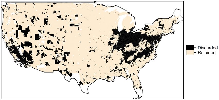
data for estimation; 4) minimizing parametric assumptions; and 5) accounting for the simultaneous effect of
multiple pollutants and thereby capturing any synergistic effects. However, to avoid extrapolation and heavy
reliance on parametric modeling assumptions, our methods exclude some areas from the analysis, thereby
producing conservative yet data-driven estimates of the health impacts of the regulation.
Matching is one of the most commonly used approaches to estimate causal effects (Ho et al., 2007; Stuart,
2010). Machine learning procedures have emerged more recently as a tool for causal inference (Hill, 2011;
Hahn et al., 2017; Louizos et al., 2017). Both have primarily been used to estimate average treatment effects
in settings with a binary treatment, with recent limited extensions to the continuous exposure setting (Kreif
et al., 2015; Wu et al., 2018). To our knowledge, neither approach has been used to do estimation in the
context of a multivariate continuous treatment (the pollution exposures in our setting). To estimate the
TEA, we develop both a matching method and an adaptation of the Bayesian Additive Regression Trees
(BART) algorithm (Chipman et al., 2010) to accommodate multivariate continuous treatments.
In Section 2, we discuss the air pollution and Medicare data that motivate our methodological devel-
opments. In Section 3, we formally introduce the TEA and identifying assumptions, and we present our
matching and machine learning methods for TEA estimation. Section 4 describes simulations conducted to
evaluate the performance of these methods. In Section 5, we apply these methods to investigate the health
impacts of the CAAA. Finally, we conclude with a summary and discussion of our findings in Section 6.
2 Data
In this paper, we focus on the number of health events prevented due to CAAA-attributable changes in
two major pollutants– PM2.5 and O3 . These two pollutants are known to have large health impacts. We
have obtained state-of-the-art factual (with-CAAA) and counterfactual (no-CAAA) gridded PM2.5 and O3
exposure estimates for the continental US in the year 2000. PM2.5 exposures (both factual and counter-
factual) are measured in µg/m3 and represent annual averages, while O3 exposures are measured in parts
per billion (ppb) and represent warm season averages. Our factual pollution exposure estimates come from
so-called hybrid models which combine ground monitor data, satellite data, and chemical transport modeling
to estimate exposures on a fine grid across the US. The factual PM2.5 exposure estimates employed here are
introduced in van Donkelaar et al. (2019) and are produced at approximately 1 km2 grid resolution. Our
factual O3 exposure estimates were developed by Di et al. (2017), also at 1 km2 grid resolution.
We employ the year-2000 counterfactual gridded PM2.5 and O3 exposure estimates for the continental
US from the EPA’s Second Section 812 Prospective Analysis (hereafter called the Section 812 Analysis), its
most recent cost-benefit analysis of the CAAA (US EPA, 2011). To produce these, gridded hourly emissions
inventories were first created for the counterfactual (no-CAAA) scenario in 2000, representing estimated
emissions with scope and stringency equivalent to 1990 levels but adjusted to economic and population
changes in 2000. Note that this approach to creating counterfactual emissions inventories assumes that 1)
in the absence of the CAAA, no new emissions regulations would have been implemented in the US between
1990 and 2000 and 2) in the absence of the CAAA, the scope and stringency of US emissions would not
have increased. We anticipate that in reality these assumptions would slightly bias the emissions estimates
in opposite directions; thus, we expect that they balance each other out to create a realistic counterfactual
emissions scenario. The emissions inventories were fed into atmospheric chemistry modeling software to
produce estimates of counterfactual annual average PM2.5 at 36 km2 grid resolution, and counterfactual
warm season O3 at 12 km2 grid resolution. For more detail on the creation of the counterfactual exposure
estimates, see US EPA (2011). We note that factual exposure estimates were also produced for the EPA’s
Section 812 Analysis in an analogous manner to the counterfactual exposures. For a discussion of why we
have chosen to use factual exposures from the hybrid models instead, see Section 2 of the Supplementary
Materials.
We use area-weighting to aggregate the gridded PM2.5 and O3 values to zip codes, in order to merge it with
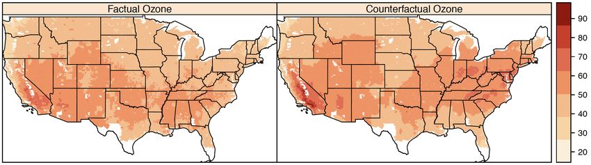
the Medicare data. See the zipcode maps of the factual and counterfactual PM2.5 and O3 data in Figure 1.
Throughout the paper, we make the strong assumption that the observed and counterfactual pollution levels
are known or estimated without error, because current limitations in air quality modeling impede reliable
3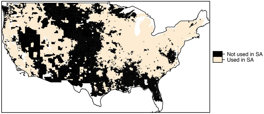
Figure 1: Maps of estimated year-2000 zipcode level factual and counterfactual annual average PM2.5 levels
in µg/m3 and warm season average O3 levels in parts per billion (ppb). The factual pollutant values are
estimates of the true exposures with the CAAA. The counterfactual values reflect the anticipated pollutant
exposures under the emissions scenario expected without the CAAA.

quantification of uncertainties (Nethery and Dominici, 2019). This is a commonly used assumption in air
pollution epidemiology, and we discuss the implications and potential impacts in Section 6.
    We construct datasets containing records for all Medicare beneficiaries in the continental US for the
years 2000 and 2001. Medicare covers more than 96% of Americans age 65 and older (Di et al., 2017).
Because cross-zipcode moving rates are low in the Medicare population (Di et al., 2017; Abu Awad et al.,
2019), we make the assumption that, for each of the 2000 and 2001 cohorts, subjects were exposed to
the year-2000 pollution levels of their zipcode of residence. Zipcode counts of mortality, cardiovascular
hospitalizations, and dementia-related hospitalizations in each cohort will serve as the outcomes in our
analysis. For detailed information about how these counts were constructed, including the ICD-9 codes
used to classify hospitalizations, see Section 2 of the Supplementary Materials. We selected these health
outcomes on the basis of previous literature associating each of them with air pollution (Pope III et al.,
2002; Moolgavkar, 2003; Brook et al., 2010; Power et al., 2016). We also compute the size of the Medicare
population in each zipcode in each year so that rates of each health event can be computed (e.g. count of
mortalities in the Medicare population in the zipcode in year 2000/total Medicare population in the zipcode
in year 2000).
    Finally, a set of potential confounders of pollution and health relationships is constructed. Confounder
data come from the 2000 US census. All confounders are zipcode-aggregate features that reflect all residents
of the zipcodes, not only Medicare beneficiaries. They are percent of the population below the poverty
line (poverty), population density per square mile (popdensity), median value of owner-occupied properties
(housevalue), percent of the population black (black), median household income (income), percent of housing
units occupied by their owner (ownhome), percent of the population hispanic (hispanic), and percent of the
population with less than a high school education (education).

                                                     4
3 Methods
3.1 Estimand and Identifying Assumptions
In this section, we propose a causal inference estimand to measure the difference in the number of health
events in a given year under the regulation and no regulation scenarios, and we lay out the identifying
assumptions. The units of analysis for our case study of the CAAA will be zipcodes, but throughout
this section we use the term units to emphasize the generality of the approach to any areal units. Let
Yi denote the count of health events observed in unit i, i = 1, ..., N , and Pi the at-risk population size
in unit i. Then let Yi∗ = PYii be the event rate. While our estimand involves counts, we must conduct
modeling with rates instead of counts when at-risk population sizes vary. Let X i denote a vector of observed
confounders of the relationship between pollution and the health outcomes under study, as well as any
factors besides the observed pollutants which were impacted by the regulation. Let T i denote the Q-length
vector of continuous pollutant exposure measurements for unit i, where Q is the number of pollutants
under consideration (annual/warm season averages), and we assume that T has compact support over a
Q-dimensional hyperrectangle, Z, which is a subspace of RQ . T i , the vector of pollutant exposure levels,
will serve as the “treatment” variable in our causal inference framework.
We develop our approach within the potential outcomes framework of Rubin (1974). Recall that we will
make use of both the factual and counterfactual pollution levels for each unit. Then let Yi (T = t1i ) be
the number of health events that unit i would experience under its observed pollutant values (t1i ) in the
factual scenario of regulation implementation. Let Yi (T = t2i ) be the number of health events that unit i
would experience under its counterfactual pollution levels (t2i ) in the no-regulation scenario, with all other
features of the unit identical to the observed ones. For each unit, Yi (T = t1i ) is observed and Yi (T = t2i ) is
unobserved. These potential outcomes can be constructed under the stable unit treatment value assumption
(SUTVA) (Rubin, 1980). SUTVA requires that the health effect of a given treatment (pollution) level is the
same no matter how that treatment level is arrived at, and that one unit’s pollution level does not affect
the number of health events in another unit (the later is known as the no interference assumption). The
former assumption could be violated if, for instance, certain sources of pollution are more toxic than others.
No interference is likely to be a strong assumption (Zigler et al., 2012; Zigler and Papadogeorgou, 2018),
as most individuals are regularly exposed to the pollution levels in areas other than their area of residence,
which could impact their health. More discussion of this assumption is provided in Sections 5 and 6.
Before formalizing the TEA, we emphasize that the TEA is designed to quantify the health impacts
of the regulation only through resultant changes in the pollutants in T , while holding all other measured
features fixed at the observed levels (under the regulation). The TEA characterizes a counterfactual scenario
in which the only changes from the observed with-regulation scenario are the pollution exposures, and
compares the number of health events in this counterfactual scenario and the observed one. We explain the
motive behind this estimand. Previous causal inference analyses (Zigler et al., 2012, 2018) have targeted
the effects of air pollution regulations on health both via the resultant changes in pollutant exposures
(associative effects) and via other intermediates (dissociative effects). These studies investigated an element
of the CAAA, the NAAQS non-attainment designations, which impacted some locations and not others,
providing variation in attainment status and observed health outcome data under both the attainment and
non-attainment scenarios. These data enabled the estimation of both associative and dissociative effects.
Here we instead wish to evaluate a larger regulation which had “universal” impacts in areas under its purview
(hereafter referred to as a universal regulation). We do not observe any health outcome data whatsoever
under the no-regulation scenario. With this limitation, our analysis must rely entirely on the observed
outcome data under regulation. Because the only information we have about the no-regulation scenario is
the counterfactual pollutant exposures, it is only through these pollutants that the observed health outcome
data can inform estimation of the health outcomes in the no-regulation scenario. Thus these data do not
allow any investigation of dissociative effects, which is why we have defined the TEA as the effect of the
regulation only through the resultant changes in the pollutants in T . The Section 812 Analysis also estimates
health effects exclusively through regulation-attributable changes in pollutants. Previous studies have found
positive dissociative health impacts of regulations (Zigler et al., 2012). If such effects exist, the TEA will
5under-represent the total number of health events prevented by the regulation.
Now invoking the notation laidPNout above, the number of health events prevented due to regulation-
induced changes in pollutants is i=1 Yi (T = t2i ) − Yi (T = t1i ). Because Yi (T = t2i ) is unobserved for all
i, we instead focus our analysis around the following estimand:
N
X
τ= E(Y (T = t2i )|X i ) − Yi (T = t1i )
i=1
τ is the TEA. With Yi (T = t1i ) observed for all i, we only need to estimate E(Y (T = t2i )|X i ) for each i
to obtain an estimate of the TEA. Note that this quantity is conditional on X i , formalizing our statement
above that, in using the TEA to evaluate a regulation, we are making the assumption that the only factor
that would have been different in the no-regulation scenario is the pollutant exposures. Moreover, this
causal estimand is unique because it captures the health effects due to changes in multiple continuous
pollutants simultaneously. This feature provides an important improvement over traditional regulation
health impact analyses, where health impacts are estimated separately for each pollutant. Analyzing each
pollutant separately is challenging, as estimates can be biased when pollution exposures are correlated, and
may fail to capture synergistic effects.
We now present the assumptions needed to identify E(Y (T = t2i )|X i ) from the observed data. These
assumptions are extensions of those of Wu et al. (2018).
Assumption 1 (A1) Causal Consistency: Yi (T = t) = Yi if T i = t
The causal consistency assumption states that the observed outcome should correspond to the potential
outcome under the observed treatment value.
Assumption 2 (A2) Weak Unconfoundedness: Let Ii (t) be an indicator function taking value 1 if T i = t and
0 otherwise. Then weak unconfoundedness is the assumption that Ii (t) ⊥
⊥ Yi (T = t)|X i .
The weak unconfoundedness assumption was introduced by Imbens (2000) and is commonly used for
causal inference with non-binary treatments. In our context, it says that assignment to treatment level t
versus any other treatment level is independent of the potential outcome at treatment t conditional on the
observed confounders.
Assumption 3 (A3) Overlap: For each {t2i , xi }, 0 < P (T = t2i |X = xi ).
The overlap assumption in this context differs slightly from the overlap (or positivity) assumption in clas-
sic causal inference analyses. It says that, for each unit’s set of counterfactual treatment and confounders, the
probability of observing that treatment and confounder level together is greater than zero. This ensures that
we are not considering counterfactuals outside the space of feasible treatment and confounder combinations.
Assumption 4 (A4) Conditional Smoothness: Let Θt = [t1 − δ1 , t1 + δ1 ] × · · · × [tQ − δQ , tQ + δQ ], tq represents
the qth element of t, and δ1 , ..., δQ are positive sequences tending to zero. Then smoothness is the assumption
that
lim E(Y |X, T ∈ Θt ) = E(Y |X, T = t)
δ1 ,...,δQ →0
This multidimensional smoothness assumption is needed due to the continuous nature of the multivariate
treatments, which means that we will never have T = t exactly and must instead rely on T within a small
neighborhood of t.
6Using these four assumptions, we show that E(Y (T = t2i )|X i ) can be identified from observed data.
E(Y (T = t2i )|X i ) = E(Y (T = t2i )|X i , T = t2i ) (by A2)
= E(Y |X i , T = t2i ) (by A1) (1)
= lim E(Y |X i , T ∈ Θt2i ) (by A4)
δ1 ,...,δQ →0
The expectation in the bottom line of equation 1 can be estimated from observed data for small, fixed values
of δ1 , ..., δQ .
In the next two sections, we introduce methods to perform this estimation with the data described
in Section 2. Before doing so, we clarify a few additional assumptions that will be relied upon in order
to interpret a TEA estimate as the number of health events avoided due to the regulation-attributable
changes in pollutants. These assumptions, which are not common in causal inference analyses, are needed
in the universal regulation scenario due to the complete reliance on observed data under the regulation
for estimation. First, we must assume that each of the following relationships would be the same in the
regulation and no-regulation scenarios: (1) the pollutant-outcome relationships, (2) the confounder-outcome
relationships, and (3) the pollutant-confounder relationships. Second, we must assume that no additional
confounders would be introduced in the no-regulation scenario.
3.2 Matching Estimator of the TEA
In this section, we introduce a causal inference matching procedure to estimate E(Y |X i , T ∈ Θt2i ) (and
thereby the TEA). In Section 3 of the Supplementary Materials, we show that the estimator is consistent,
and we describe a bootstrapping approach that can be used to compute uncertainties. The idea behind our
matching approach is simple: we will find all units with observed pollutant levels approximately equal to
t2i and confounder levels approximately equal to X i , and we will take the average observed outcome value
across these units (plus a bias correction term) as an estimate of E(Y |X i , T ∈ Θt2i ).
Let ω be a Q-length vector of pre-specified constants and ν be a pre-specified scalar. For a column
vector b, |b| denotes the component-wise absolute value and ||b|| = (b0 Ab)1/2 , with A a positive semidefinite
matrix. In practice, A will be a covariance matrix so that ||b1 − b2 || is the Mahalanobis distance. We let
ϕ(i) denote the set of indices of the units matched to unit i. Then
ϕ(i) = {j ∈ 1, ..., N : |t2i − t1j | ≺ ω ∧ ||X i − X j || < ν}
In the first condition here, we are carrying out exact matching within some tolerances ω on the pollution
variables, so that the units matched to unit i have observed pollution levels (t1j ) almost equal to the
counterfactual pollution levels for unit i (t2i ). This ensures that the matched units have observed pollution
values within a small hyperrectangle around t2i , i.e. T ∈ Θt2i . The second condition carries out Mahalanobis
distance matching within some tolerance ν on the confounders, so that all matched units have confounder
values approximately equal to the confounder values for unit i. We use separate procedures for matching on
the pollution and the confounder values so that we can exercise more direct control over the closeness of the
matches on pollution values. Literature on choosing calipers in standard matching procedures (Lunt, 2013)
and identifying regions of common support in causal inference (King and Zeng, 2006) may provide insight
into how to specify ω and ν. All units that meet the above conditions are used as matches for unit i, thus
each i is allowed to have a different number of matches, Mi . Matching is performed with replacement across
the i. Then, we estimate E(Y |X i , T ∈ Θt2i ) as
Pi X ∗
Ê(Y |X i , T ∈ Θt2i ) = Yk (2)
Mi
k∈ϕ(i)
We also test varieties of this matching estimator with bias corrections following Abadie and Imbens
(2011), because bias corrected matching estimators can provide increased robustness. Let µ̂(t2i , X i ) be a
7regression-predicted value of Y conditional on t2i and X i . Then the bias corrected estimator has the form
1 X
Ê(Y |X i , T ∈ Θt2i ) = (Yk∗ Pi + µ̂(t2i , X i ) − µ̂(t2i , X k ))
Mi
k∈ϕ(i)
While asymptotically matches will be available for all units (as a result of the overlap assumption, A3),
in practice there will likely be some units for which no suitable matches can be found in the data. Let
s = 1, ..., S index the units for which 1 or more matches was found. Instead of τ , in finite sample settings
we will generally estimate
XS
τ∗ = E(Y |X s , T ∈ Θt2s ) − Ys (T = t1s )
s=1
by plugging in Ê(Y |X s , T ∈ Θt2s ) for E(Y |X s , T ∈ Θt2s ). This discarding of unmatched units is often called
“trimming” and the remaining S units called the trimmed sample. This trimming is done to avoid using
extrapolation to estimate counterfactual outcomes in areas of the treatment/confounder space that are far
from the observed data. Such extrapolation can produce results that are highly biased or model-dependent.
3.3 BART for TEA Estimation
In this section, we propose an alternative approach to estimation of the TEA relying on machine learning.
Machine learning procedures are typically applied in causal inference as a mechanism for imputation of
missing counterfactual outcomes. BART (Chipman et al., 2010) is a Bayesian tree ensemble method. Several
recent papers have shown its promising performance in causal inference contexts (Hill, 2011; Hahn et al.,
2017).
The
PJgeneral form of the BART model for a continuous outcome Y and a vector of predictors X is
Y = j=1 g(X; Tj , Mj ) + , where j = 1, ..., J indexes the trees in the ensemble, g is a function that sorts
each unit into one of a set of mj terminal nodes, associated with mean parameters Mj = {µ1 , ..., µmj }, based
on a set of decision rules, Tj . ∼ N (0, σ 2 ) is a random error term. BART is fit using a Bayesian backfitting
algorithm. For estimation of average treatment effects (ATE) in a binary treatment setting, BART is fit to
all the observed data and used to estimate the potential outcome under treatment and under control for each
unit (Hill, 2011). The average difference in estimated potential outcomes is computed across the sample to
obtain an ATE estimate.
We invoke BART similarly to estimate the TEA, inserting the rates as the outcome. For clarity in this
section, we use the notation Yi∗ as the observed outcome rate under the factual pollution levels and Ȳi∗ as
the missing counterfactual outcome rate under the counterfactual pollution levels. PJ Boldface versions denote
the vector of all outcomes. We fit the following BART model to our data: Yi∗ = j=1 g(t1i , X i ; Tj , Mj ) + i .
We collect H posterior samples of the parameters from this BART model, referred to collectively as θ. For
a given posterior sample h and for each unit i, we collect a sample from the posterior predictive distribution
∗(h)
of Ȳi∗ , p(Ȳi∗ |Y∗ ) = p(Ȳi∗ |Y∗ , θ)p(θ|Y∗ )dθ. Denote this posterior predictive sample Ȳi . We use these
R
N ∗(h)
to construct a posterior predictive sample of τ as τ (h) = − Yi∗ )Pi . We then estimate τ̂ =
P
PH i=1 (Ȳi
1 (h)
H h=1 τ , i.e. the posterior mean. To relate this back to the notation of the previous section, note that
PH ∗(h)
this is equivalent to estimating Ê(Y |X i , T ∈ Θt2i ) = H1 h=1 Ȳi for all i. A 95% credible interval is
(h)
formed with the 2.5% and 97.5% percentiles of the τ .
Recall that, with the matching estimator, units for which no matches can be found within the pre-
specified tolerances are trimmed to avoid extrapolation, so that we estimate τ ∗ rather than τ . BART does
not automatically identify units for which extrapolation is necessary to estimate counterfactual outcomes.
Hill and Su (2013) proposed a two-step method to identify units for trimming with BART which could be
adapted for use here. In our simulations and analyses, to ensure comparability of the results from BART
and matching, we fit the BART model to the entire dataset but, in estimating the TEA, we omit the same
set of units that are trimmed with matching.
84 Simulations
In this section, we generate synthetic data mimicking the structure of our real data and test the following
methods for estimating τ ∗ : our matching procedure with various types of bias correction, our BART proce-
dure, and a simple Poisson regression. In these simulations, we let N = 5, 000 and Q = 2, with one pollutant
simulated to mimic PM2.5 (in µg/m3 ) and the other O3 (in parts per million). Specifically, the observed
0
pollutants are generated as follows: t1i ∼ M V N (µ, Σ), µ = [12.18 0.05] , Σ = diag([7.99 0.0001]). Then,
using t1i , we generate the counterfactual pollution levels as t2i = t1i + z i , z i = [z1i z2i ], z1i ∼ U nif (0, 7.08)
and z2i ∼ U nif (0, 0.03). The result is that the counterfactual pollutant levels are always larger than the
observed pollutant levels, but the magnitudes of the differences vary across units and at appropriate scales
for each pollutant.
We use the exposure values to generate five confounders, X1i , ..., X5i . We let Xhi = t01i αh + hi , where
hi ∼ N (0, σh2 ). In addition to the exposures and confounders, we also generate four random variables used
as “unobserved” predictors of Y , i.e. we use them to generate Y but do not include them in the estimation
procedures (they are not confounders because they are not related to exposure). In our real data analysis,
there are likely many unobserved predictors of the health outcomes considered (but hopefully no unobserved
confounders), thus it is important to evaluate our methods under such conditions.
In each simulation, we generate Yi ∼ P oisson(λi ), with λi a function of the observed exposures, con-
founders, and predictors. We also generate an expected counterfactual outcome for each unit, λcf i using the
same functional form but substituting the counterfactual exposure values for the observed exposure values.
We consider three different functional forms for λi , and we refer to the different structures as S-1, S-2, and
S-3. S-1 uses the most complex form to construct Y , involving strong non-linearities and interactions both
within and across the exposures and confounders. S-2 is slightly less complex, with exposure-confounder
interactions excluded. Finally, in S-3 all relationships are linear. See the model forms and parameter values
used in each simulation in Section 5 of the Supplementary Materials. Parameter values are chosen so that
the distribution of Y is similar to the distribution of our outcomes in the Medicare data.
With these data we first perform matching to determine which units have suitable matches for their
t2i in the data and will therefore contribute to the estimation of τ ∗ . Within each of the three simulation
scenarios, we set ν = 1.94, which is approximately the 10th percentile of the Mahalanobis distances between
all the units in the data, and consider three different specifications of ω, the tolerances for the pollutant
matches. We use 10%, 15%, and 25% of the standard deviations of the counterfactual pollutant distributions,
resulting in ω = [0.35 0.001], ω = [0.53 0.002], and ω = [0.88 0.003]. Following matching, we estimate
three variations of the matching estimator. The first is the simple matching estimator given in equation 2
(Match 1). The second is this matching estimator plus a bias correction from a Poisson regression with linear
terms, i.e. log(λi ) = β0 + t01i X 0i β (Match 2). The third is the matching estimator with a bias correction
from a Poisson regression in which the forms of the exposures and confounders are correctly specified (Match
3). We also apply BART as described in Section 3.3, fitting the BART model to all the data but estimating
the TEA with only the units retained after matching. We also compare these methods to a simple Poisson
regression. We fit a Poisson regression with all exposures and confounders included as linear terms (PR 1)
and a Poisson regression model in which the forms of the exposures and confounders PSare correctly specified
(PR 2). We compare each estimate to the true TEA in the trimmed sample, τ ∗ = s=1 λcf s − λs .
Table 1 contains the simulation results. It shows the proportion of units retained after trimming, the
ratio of the true trimmed sample TEA to the true whole sample TEA, and the percent bias and 95% confi-
dence/credible interval coverage (in parentheses) for each method in each simulation. Across all simulations,
substantial portions of the sample are being trimmed (37%-58%). These trimmed units account for a dis-
proportionately high amount of the TEA, as τ ∗ /τ is generally much smaller than S/N . This reflects the
scenario we would expect in our real data, because the units with the highest counterfactual pollution levels
are likely to have the largest effect sizes, yet these units are unlikely to be matched since we may observe
few or no pollution exposures as high as their counterfactuals.
In all cases either Match 3 or PR 2, the methods with correct model specification, achieves the best
performance. However, in general we do not know the correct functional form of the model, therefore a
9Table 1: Percent absolute bias (95% confidence/credible interval coverage) of the following methods in
estimation of τ ∗ in 200 simulations: matching with no bias correction (Match 1), matching with a linear bias
correction (Match 2), matching with correctly specified bias correction (Match 3), BART, Poisson regression
with linear terms (PR 1), correctly specified Poisson regression (PR 2). ω refers to matching tolerances
on pollutants, i.e. 0.1 means that matches are restricted to be within 0.1 standard deviations for each
pollutant. S/N is the proportion of the sample retained after trimming, and τ ∗ /τ is the ratio of the true
trimmed sample TEA to the true whole sample TEA.
ω S/N τ ∗ /τ Match 1 Match 2 Match 3 BART PR 1 PR 2
0.1 0.42 0.22 0.23 (0.19) 0.06 (0.98) 0.02 (0.99) 0.05 (0.82) 0.76 (0.00) 0.03 (0.72)
S-1
τ = 60577 0.15 0.54 0.30 0.30 (0.00) 0.14 (0.65) 0.01 (0.95) 0.07 (0.54) 0.62 (0.00) 0.02 (0.84)
0.25 0.67 0.42 0.39 (0.00) 0.22 (0.10) 0.04 (0.79) 0.08 (0.44) 0.50 (0.00) 0.02 (0.88)
0.1 0.42 0.22 0.31 (0.05) 0.08 (0.98) 0.02 (1.00) 0.07 (0.71) 0.85 (0.00) 0.04 (0.73)
S-2
τ = 49610 0.15 0.54 0.31 0.38 (0.00) 0.16 (0.62) 0.02 (0.96) 0.10 (0.38) 0.69 (0.00) 0.02 (0.86)
0.25 0.67 0.43 0.48 (0.00) 0.25 (0.09) 0.04 (0.78) 0.11 (0.35) 0.57 (0.00) 0.02 (0.88)
0.1 0.42 0.32 0.42 (0.77) 0.01 (0.98) - 0.13 (0.97) 0.03 (0.90) -
S-3
τ = 5321 0.15 0.54 0.42 0.53 (0.60) 0.17 (0.87) - 0.22 (0.94) 0.13 (0.84) -
0.25 0.67 0.56 0.54 (0.44) 0.15 (0.90) - 0.23 (0.94) 0.15 (0.89) -
comparison of the other methods is more relevant to real data. Among the remaining methods, we generally
see that as ω increases, the bias of the TEA estimates increase. This is consistent with expectations, as a
larger ω allows matches with more distant exposure values, which can lead to inappropriate extrapolation.
Match 1 and PR 1 generally are not reliable, with bias consistently greater than 30% and poor coverage.
Thus, we focus on a comparison of BART and Match 2.
BART has the smallest bias in every simulation within S-1 and S-2. This is consistent with previous
research, which has shown BART to accurately capture complex functional forms. However, BART and
other tree-based methods often struggle with simple linear relationships. This is reflected in the results of
S-3, where Match 2 achieves smaller bias.
The takeaways regarding coverage are more complicated. We see that, in all simulations with ω = 0.1 and
ω = 0.15, Match 2 provides superior coverage to BART. However, as the matching tolerance is increased,
leading to greater bias, the coverage of Match 2 declines more rapidly than BART’s coverage. This is
evidenced by BART’s superior coverage in all simulations with ω = 0.25.
These results demonstrate the trade-offs that must be considered when choosing the matching tolerances,
or more generally when choosing which units to trim. This issue is particularly salient in this setting because
our estimand of interest, the TEA, is a sum rather than an average. When computing a sum, the removal of
one unit is likely to impact the estimate more than the removal of the same unit when computing an average.
The stricter the tolerances, the more units are dropped from the analysis and, generally, the more distant τ ∗
will grow from τ . Therefore, the estimated TEA is less and less likely to reflect the population of interest. In
our context where greater pollution exposure is unlikely to have protective effects on health, and where most
of the counterfactual pollution levels are greater than the factual ones (i.e. Y (T = t2i ) − Y (T = t1i ) > 0),
we anticipate that stricter tolerances and the trimming of more units will lead to underestimation of the
TEA. However, stricter tolerances reduce the potential for extrapolation and generally give estimates of τ ∗
with lower bias. The selection of these tolerances should be considered carefully in the context of each data
application. In the simulated data tolerances of 0.1 and 0.15 standard deviations of each pollutant gave
reliable results.
5 Application
We return now to the real data described in Section 2. Because the purpose of the CAAA was to reduce
air pollution, we would expect the counterfactual (no-CAAA) pollution exposures to be higher than fac-
10tual (with-CAAA) pollution exposures in most zipcodes; however, the CAAA resulted in a complex set of
regulations that could have led to decreases in some areas and increases in others. In our data, in 27% of
the zipcodes the factual PM2.5 and/or O3 exposure estimate is larger than the corresponding counterfactual
estimate, indicating that the CAAA increased exposure to at least one of the pollutants. See Section 5 of the
Supplementary Materials for a map showing the locations of these zipcodes. This could reflect real increases
in pollution exposures due to the CAAA or it could be partially due to differences in the pollution exposure
modeling used to produce the factual and counterfactual estimates. In our primary analysis (PA), to be
conservative we include these zipcodes with one or both factual pollutants larger than the corresponding
counterfactual, and we also perform a sensitivity analysis (SA) in which they are removed. In the SA, we
allow all zipcodes to serve as potential matches but the TEA’s sum is only taken across zipcodes with both
factual pollutant estimates smaller than the corresponding counterfactual estimate.
Within each of the PA and SA, we conduct separate analyses to estimate the health impacts in years
2000 and 2001 due to CAAA-attributable changes in pollution exposures in the year 2000. Prior to analysis,
we remove any zipcodes with missing data or with zero Medicare population. For the year 2000, the sample
size following these removals is N = 28, 155 zipcodes (SA: N = 20, 432). All descriptive statistics provided
are from the year 2000 data. Figures for 2001 deviate little, if at all, due to year-specific missingness and
Medicare population size. For each year’s data we apply BART, matching with a linear bias correction,
and a Poisson regression with linear terms to estimate the TEA for mortality, cardiovascular disease (CVD)
hospitalizations, and dementia hospitalizations. We apply these methods using the rates of each health
outcome (yearly event count/population size).
We first apply matching to the data, with 50 bootstrap replicates and with tolerances ω = [0.56 0.77]
and ν = 2.12. As in the simulations the ω values are 0.1 standard deviations of each counterfactual
pollutant distribution, and ν is approximately the 10th percentile of the Mahalanobis distances between
all the confounders in the data. These tolerances lead to trimming of 10,313 zipcodes (SA: 8,936), leaving
S = 17, 842 zipcodes (SA: S = 11, 496) for estimation of the TEA. The portion of the full dataset retained
to estimate the TEA, S/N = 0.63 (SA: S/N = 0.56), is similar to that in the simulations. As described in
Sections 3 and 4, we fit the BART and Poisson regression to the entire sample but then only include the
units retained after trimming for estimation of the TEA.
The total Medicare population in the zipcodes retained after trimming is 15,573,107 (SA: 10,096,548).
Table 2 shows the means and standard deviations of the Medicare population size, Medicare health outcome
rates, exposures and confounders in the full dataset, among the discarded/trimmed zipcodes, and in the
retained/untrimmed zipcodes used for estimation for the PA. In Section 5 of the Supplementary Materials,
we provide a map showing the locations of the discarded and retained zipcodes after trimming for the PA, and
an analog of Table 2 for the SA. The discarded zipcodes are primarily in the midwest, where Figure 1 shows
some of the highest counterfactual pollutant levels (this result is consistent with our simulation takeaways
in Section 4), and in major east and west coast cities. Notably, the discarded zipcodes have larger average
population size and higher average pollutant exposures (both factual and counterfactual) than the full
dataset. As discussed in Section 4, this is likely due to the fact that we have sparse observed data at very
high exposure levels and therefore it is difficult to find matches for zipcodes with very high counterfactual
exposures (which also tend to be the more highly populous zipcodes). We would also expect that many of the
largest health benefits of the CAAA may have come in zipcodes with large populations and whose no-CAAA
exposures would have been very high, thus our results are likely to be underestimates of the effects in the
whole population.
The results of both the PA and SA appear in Figure 2. We first note that the results of the PA and
SA are highly similar, indicating that the zipcodes for which one or both of the factual pollutant exposures
are larger than the counterfactual have little impact on the analysis. Matching and BART find limited,
although somewhat inconsistent, evidence of effects on mortality. Only the BART analysis for 2001 detects
an effect, estimating approximately 10,000 mortalities prevented in the retained zipcodes, with the lower
credible interval limit just exceeding zero. For CVD and dementia hospitalizations, all the methods yield
large positive point estimates, i.e., large estimates of the number of events avoided in the specified year
due to CAAA-attributable pollution changes in 2000. The estimates from BART and matching suggest
11Table 2: Average (and standard deviation) of Medicare population size, Medicare health outcome rates,
pollutant exposures and confounders in the full dataset, only the discarded/trimmed zipcodes, and the
retained/untrimmed zipcodes used for estimation.
Full Dataset Discarded Units Retained Units
Population size 1091.76 (1514.94) 1470.52 (1797.91) 872.83 (1273.76)
Mortality (rate per 1,000) 52.22 (21.29) 52.79 (21.8) 51.89 (20.99)
Dementia (rate per 1,000) 16.69 (14.27) 17.48 (17.19) 16.23 (12.25)
CVD (rate per 1,000) 72.35 (31.22) 70.43 (33.64) 73.45 (29.68)
Factual PM2.5 (µg/m3 ) 10.51 (3.76) 12.26 (3.34) 9.5 (3.61)
Factual O3 (ppb) 46.92 (6.15) 47.22 (6.76) 46.75 (5.76)
Counterfactual PM2.5 (µg/m3 ) 14.5 (5.62) 18.5 (5.85) 12.18 (3.92)
Counterfactual O3 (ppb) 53.3 (7.74) 57.7 (8.33) 50.76 (6.06)
poverty (proportion) 0.11 (0.1) 0.12 (0.12) 0.11 (0.08)
popdensity (per mi2 ) 1146.31 (4426.27) 2437.78 (6989.55) 399.81 (1076.25)
housevalue (USD) 103528.58 (82347.49) 131038.42 (114351.7) 87627.39 (49523.45)
black (proportion) 0.08 (0.16) 0.11 (0.2) 0.06 (0.13)
income (USD) 40222.76 (16041.13) 43952.52 (20441.86) 38066.89 (12322.53)
ownhome (proportion) 0.75 (0.15) 0.71 (0.2) 0.78 (0.1)
hispanic (proportion) 0.06 (0.12) 0.08 (0.16) 0.05 (0.09)
education (proportion) 0.38 (0.18) 0.4 (0.2) 0.38 (0.16)
that approximately 23,000 dementia hospitalizations and approximately 50,000 CVD hospitalizations were
avoided in each year. None of the 95% confidence/credible intervals for these outcomes overlaps zero,
providing strong evidence of an effect. The Poisson regression gives all positive and statistically significant
TEA estimates, with the significance attributable to extremely narrow confidence intervals. However, the
simulation results suggest that these results are likely untrustworthy.
Air pollution literature accumulated over the past 20 years has provided strong evidence to support a
causal relationship between long-term PM2.5 exposure and mortality (US EPA, 2009). This relationship has
also been reported in a recent analysis of Medicare data (Di et al., 2017). One major difference in our study
compared to previous cohort studies examining long-term PM2.5 exposure and mortality is that we are using
zipcode aggregated data while they use individual level data. The use of individual level data allows for
adjustments for individual level features, while the use of aggregated data does not. Therefore, results from
individual level data are often preferred. Given the complex nature of mortality, our inability to adjust for
individual level factors may make mortality rates appear too noisy to detect pollution effects. Our results are
consistent with the recent findings of Henneman et al. (2019) who investigate coal emissions exposures and
health outcomes at the zipcode level in the Medicare population. They also find limited effects on mortality
but strong evidence of harmful effects on CVD hospitalizations.
To demonstrate how the approach introduced in this paper can be used in conjunction with traditional
health impact assessments, we provide the EPA’s Section 812 Analysis estimates for the number of mortalities
and CVD hospitalizations prevented in the year 2000 due to the CAAA in Section 4 of the Supplementary
Materials. We also provide additional context to clarify how their estimates can be compared to ours. In
short, our approach yields a conservative set of results entirely supported by real, population-level health
outcome data. Our results also account for any synergistic effects of the pollutants on health. The traditional
approach used in the Section 812 analysis relies on 1) health effect estimates from cohort studies which allow
for extensive confounding adjustment but may not fully reflect the population of interest; and 2) a stronger set
of modeling assumptions which, while unverifiable, allows for the number of events avoided to be estimated
in areas with no support in the real data. Considering the distinct strengths and limitations of our approach
and the traditional approach, the results of both types of analysis are likely to provide useful insights about
the health impacts of large air pollution regulations.
Finally, we note that in order to interpret our results here as causal, we must be willing to make the
12PA−2000 PA−2001 SA−2000 SA−2001
50000
Mortality
25000
● ●
0 ● ●
50000
Method
Dementia
● Match
25000 ●
●
● BART
●
PR
0
●
●
50000 ● ●
CVD
25000
0
Figure 2: Primary analysis (PA) and sensitivity analysis (SA) estimates and 95% confidence/credible intervals
for the TEA in the Medicare population in 2000 and 2001 due CAAA-attributable changes in PM2.5 and O3
in the year 2000. Estimation is performed using matching with a linear bias correction, BART, and Poisson
regression (PR).
strong causal identifying assumptions put forth in Section 3. The no unobserved confounding assumption
could be called into question, because we have not adjusted for potential behavioral confounders such as
smoking and obesity. However, these features may be highly correlated with features we do adjust for, e.g.
education. We also make the strong assumption of no interference. It is unclear how a violation of this
assumption would impact our results. However, this assumption has been made in most causal inference
analyses of air pollution to date (Papadogeorgou and Dominici, 2018; Wu et al., 2018).
6 Discussion
In this paper, we have introduced a causal inference approach for evaluating the health impacts of an air
pollution regulation. We developed an estimand called the TEA and proposed a matching and a machine
learning method for estimation. Both methods showed promising performance in simulations, particularly
in comparison to standard parametric approaches. We implemented these methods to estimate the TEA for
mortality, dementia hospitalizations, and CVD hospitalizations in the Medicare population due to CAAA-
attributable pollution changes in the year 2000. We found compelling evidence that CAAA-attributable
pollution changes prevented large numbers of CVD and dementia hospitalizations. Because more than one
third of the zipcodes were trimmed from our analysis to avoid extrapolation, and because the trimmed
zipcodes tend to have larger populations and larger improvements in air quality due to the CAAA, we
expect that the true number of health events avoided may be considerably larger than our estimates.
While our causal inference approach improves on the traditional approach to regulation evaluation in
many ways, there are trade-offs to be considered. In order to avoid extrapolation and strong model-
dependence, our methods discard units whose counterfactual pollution/confounder values are far outside
the observed pollution/confounder space. This often leads to discarding of units where the highest impacts
13would be expected. Our estimates tend to have small bias in estimating the effects in the trimmed sample;
however the effects in the trimmed sample may be much lower than in the entire original sample. The tradi-
tional approach to regulatory evaluation retains all units for estimation, and simply uses parametric models
to extrapolate counterfactual outcomes for units with pollutant/confounder values outside areas of support
in the observed data. This extrapolation could produce biased estimates, but it is not obvious what the
direction of that bias would be. It may be useful to apply and compare both approaches in future regulation
evaluations.
The limitations and assumptions of our methods present opportunities for future methodological ad-
vancements. In particular, approaches for causal inference with interference could be integrated from recent
work (Barkley et al., 2017; Papadogeorgou et al., 2019). Because our analyses could be affected by unob-
served spatial confounding, future work could amend our matching approach to take into account distance
between matched zipcodes (Papadogeorgou et al., 2018). We also note that, because our outcome is rate
data, BART’s normality assumption may be violated. A BART for count data has been proposed (Murray,
2017), but at the time of writing this manuscript, code was not available. Moreover, future work could extend
our approach to accommodate individual level data instead of aggregated data. Finally, our approach relies
on pollution data from different sources, i.e., factual pollution estimates from hybrid models and counterfac-
tual estimates from the EPA’s Section 812 analysis. In the Supplementary Materials, we provide extensive
justification for this choice; however, our results may suffer from incompatibility in the pollution exposure
estimates, which could be improved upon in future work.
Finally, improvements in pollution exposure data more broadly are essential to increase the reliability of
our approach. Statisticians and engineers should work together to produce nationwide factual and counter-
factual pollution exposure estimates that are increasingly spatially granular and are more tailored for this
type of analysis. These estimates should be accompanied by uncertainties, which could be taken into account
in downstream analyses to provide inference that reflects both outcome and exposure uncertainty.
7 Code
R code and instructions for reproducing these analyses is available at https://github.com/rachelnethery/
AQregulation.
8 Disclaimer
This manuscript has been reviewed by the U.S. Environmental Protection Agency and approved for publi-
cation. The views expressed in this manuscript are those of the authors and do not necessarily reflect the
views or policies of the U.S. Environmental Protection Agency.
9 Acknowledgements
The authors gratefully acknowledge funding from NIH grants 5T32ES007142-35, R01ES024332, R01ES026217,
P50MD010428, DP2MD012722, R01ES028033, and R01MD012769; HEI grant 4953-RFA14-3/16-4; and EPA
grant 83587201-0.
10 Supplementary Materials
10.1 Traditional Approaches to Health Impact Assessments for Air Pollution
Regulations
Several tools have been developed worldwide that vary in complexity to estimate the potential health impli-
cations of changes in air quality including WHO’s AirQ+, Aphekom (Improving Knowledge and Communi-
14You can also read