Assessing the performance of a Northeast Asia Japan-cantered 3-D ionosphere specication technique during the 2015 St. Patrick's day solar storm ...

Assessing the performance of a Northeast Asia
Japan-cantered 3-D ionosphere speci cation
technique during the 2015 St. Patrick’s day solar
storm
Nicholas Ssessanga (  nikizxx@gmail.com )
 Kyodai Uji: Kyoto Daigaku - Uji Campus
Mamoru Yamamoto
 Kyoto Daigaku - Uji Campus
Susumu Saito
 Electronics Navigation Research Institute

Full paper

Keywords: Ground-GNSS-STEC tomography, Ionosonde data assimilation, geomagnetic storm

Posted Date: March 15th, 2021

DOI: https://doi.org/10.21203/rs.3.rs-287515/v1

License:   This work is licensed under a Creative Commons Attribution 4.0 International License.
Read Full License

Title: Assessing the performance of a Northeast Asia Japan-cantered 3-D

ionosphere specification technique during the 2015 St. Patrick’s day solar storm

Author #1: Nicholas Ssessanga

Institution: Research Institute for Sustainable Humanosphere, Kyoto University, Uji,

Kyoto, Japan

Email: nikizxx@gmail.com

Author #2: Mamoru Yamamoto

Institution: Research Institute for Sustainable Humanosphere, Kyoto University, Uji,

Kyoto, Japan

Email: nikizxx@gmail.com

Author #3: Susumu Saito

Institution: National Institute of Maritime, Port, and Aviation Technology, Electronic

Navigation Research Institute, Tokyo, Japan

Email: susaito@enri.go.jp

Corresponding author

Correspondence to Nicholas Ssessanga

 1

Abstract

This paper demonstrates and assesses the capability of the advanced three-

dimensional (3-D) ionosphere tomography technique, during severe conditions. The

study area is northeast Asia and quasi-Japan-centred. Reconstructions are based on

Total electron content data from a dense ground-based global navigation satellite

system receiver network and parameters from operational ionosondes. We used

observations from ionosondes, Swarm satellites and radio occultation (RO) to assess

the 3-D picture. Specifically, we focus on St. Patrick’s day solar storm (17-19 March

2015), the most intense in solar cycle 24. During this event, the energy ingested into

the ionosphere resulted in Dst and Kp and reaching values ~-223 nT and 8,

respectively, and the region of interest, the East Asian sector, was characterized by a

~60% reduction in electron densities. Results show that the reconstructed densities

follow the physical dynamics previously discussed in earlier publications about storm

events. Moreover, even when ionosonde data were not available, the technique could

still provide a consistent picture of the ionosphere vertical structure. Furthermore,

analyses show that there is a profound agreement between the RO profiles/in-situ

densities and the reconstructions. Therefore, the technique is a potential candidate for

applications that are sensitive to ionospheric corrections.

Keywords

Ground-GNSS-STEC tomography; Ionosonde data assimilation; geomagnetic storm

 2

1. Introduction

In trans-ionospheric radio communication, central to the precise performance is the

ability to understand, characterize, and forecast the distribution of an irregular

transiently changing dispersive terrestrial plasma (see for example Jakowski et al.

2011; Cannon et al. 2013; Kelly et al. 2014; Eastwood et al. 2017; Yasyukevich et al.

2018; Rovira-Garcia et al. 2020). Despite the complexity of this subject, traditionally

in the past few years a simplistic horizontal distribution has been suffice, to a certain

level of accuracy, to correct for the ionospheric effects on radio signals (e.g., Saito et

al. 1998; Jakowski et al. 2012, 2011; Ohashi et al. 2013). The horizontal distribution

is mainly deducible from total electron content (TEC), a derivable quantity from

abundantly available satellite-ground radio transmissions (Otsuka et al. 2002; Ma and

Maruyama, 2003). However, as technological systems become more integrated, the

demand for high precision on trans-ionospheric signals has increased. Thus, the need

for a detailed three-dimensional (3-D) ionosphere picture. Computerized ionosphere

tomography (CIT) is a way to make 3-D (or 2-D) distribution, i.e., an analysis

technique to give height dimension from the organized multi-point measurements of

TEC. Such advanced CIT is now called ionospheric imaging and is vital in radio

communication since it provides information on the four-dimensional (time and space)

evolution of the electron density structure. An excellent review and history on some

of these techniques is found in Bust and Mitchell (2008).

The fidelity of the imaging technique depends on the accuracy of the measurements as

well as the temporal and spatial distribution of the data used in the reconstruction.

Unfortunately, in most cases, measurements are imperfect and irregular in space and

time. Besides, geometry constraints limit the observation information that can be

included in the analysis. In return, imaging or tomography analysis (inverse problems)

 3

are generally under-determined and ill-posed (Yeh and Raymund, 1991; Raymund et

al. 1994; Bust and Mitchell 2008). To have a consistent 3-D picture, a prior

information from other sources such as models is needed. The accuracy of this

information and the subject of how to best combine it with measurements has

spawned an explosion of research and suggestions (e.g., Fremouw et al. 1992; Howe

et al.1998; Rius et al. 1998; Bust et al. 2000; Tsai et al. 2002; Mitchell and

Spencer, 2003; Ma et al. 2005; Schmidt et al. 2008; Okoh et al. 2010; Seemala et al.

2014; Ssessanga et al. 2015; Chen et al. 2016; Saito et al. 2017).

To maximize the advantages of imaging techniques, reconstructions are performed on

a regional basis; wherein observations are abundant, and computation is tractable

under high spatial grid resolution settings. Over the East-Asian sector, an imaging

technique has been developed based on a regional network of dense GNSS (global

navigation satellite system) receivers and ionosondes (Saito et al. 2017, 2019;

Ssessanga et al. 2021). Figure 1 showcases the network and the horizontal resolution

settings. The vertical dimension is not illustrated in the picture but extends to a GNSS

altitude of 25,000 km (see Saito et al. 2017). The technique is a two-stage algorithm:

First GNSS STEC (slant total electron content) are used to reconstruct the ionosphere

electron density field based on constrained least-squares CIT. Second, to improve the

exactness of the reconstructed picture, CIT densities are considered as background in

an ionosonde data assimilation technique which assumes that ionosphere electron

densities are better described by a log-normal distribution. Saito et al. (2017, 2019)

and Ssessanga et al. 2021, have provided the mathematical derivation of this

algorithm together with some preliminary results showing that the algorithm performs

better than a stand-alone CIT technique. However, the authors did not specifically

provide a performance analysis of the algorithm during geomagnetically disturbed

 4

conditions. Moreover, a wide spectrum of energy injected into the ionosphere during

geomagnetic storms leads to a chaotic and non-linear ionosphere both in space and

time. Although the main phase of a storm may last for a short period, the aftermath

effects can last for many days before recovery (Prölss (1995) and Buonsanto (1999)).

Under such deviant conditions, most climate (such as international reference

ionosphere(IRI)) or physics-based models used in forecasting and nowcasting

ionospheric behaviour are rendered insufficient. Therefore, for applications that

utilize trans-ionospheric signals, a need for a data-sensitive near-real-time observation

driven algorithm is paramount. The goal of this paper is to show that the technique

suggested by Ssessanga et al. 2021, can detect electron density dynamics even during

severe storm conditions, and thus a potential candidate for near-real-time ionospheric

corrections/applications. All hyperparameters are maintained the same as published in

Saito et al. (2017, 2019) and Ssessanga et al. 2021. Section 2 gives a short

mathematical description of the technique. Section 3 presents the reconstructions‐

measurement(ionosonde) comparisons illustrating the ionosphere electron density

dynamics in connection to the ingested energy during the geomagnetic storm. It also

analyses in detail the reconstructed densities in comparison to independent

observations from Swarm satellites and radio occultation. Section 4 is the summary.

2. A brief description of the algorithm
 
Consider a required regional 3-D electron density field state ( n ) and a column vector

Y of observations within the specified grid. Then a cost function to be minimized

under constrained least-squares fit is expressed as
      
J (n) =|| An − Y + Abc n bc ||2 + || Wn + Wbc n bc ||2 (1)
 
and the solution (n ) that minimizes (1) is written as

 5

   
n = (AT A + WT W)−1 (AT (Y + Abc n bc ) − WT Wn bc ) (2)

where A is an operator that maps the electron density field state into observation

space, W is a weight matrix based on prior information and restrains the derived

electron density from exceeding a certain value (Saito et al. (2017, 2019)). Elements

superscripted with bc represent boundary conditions obtained from the NeQuick

model (Nava et al. 2008) and where λ (> 0) is a regularization parameter. In the

nutshell, the tomography analysis is based on the dense GPS-TEC data with model

empirical data normalized to vertical profile peak densities and only used to constraint

the solution (see Seemala et al. 2014). We developed a software system on a desktop

PC, and realized the realtime tomography analysis from 1-second GEONET data from

200 stations over Japan. Performance of this tomography (Saito et al. (2017, 2019))

was generally good, but limited when the F region peak densities (NmF2) appeared

below the ~270 km altitude range in October and November.

Ssessanga et al. (2021) developed an advanced version of this tomography by

incorporating two more features that provide a more realistic representation of the

ionosphere. One is the inclusion of the ionosonde parameters h'F and foF2 from the

nearby operational ionosondes. The other is the evaluation of data as logarithmic of
 
the targeted densities; whereby all the elements in random vector n are assumed to

be drawn from log-normal distributions, and then apply Gaussian statics by taking the

natural logarithm of each element ( ). That is

xi = log(ni )
 (3)

A new cost function is then formulated as follows

  1     1    
 J ( X ) = [Y − A ( X )]T R −1[Y − A( X )] + [ X − X b ]T B −1[ X − X b ]
 2 2 (4)

 6


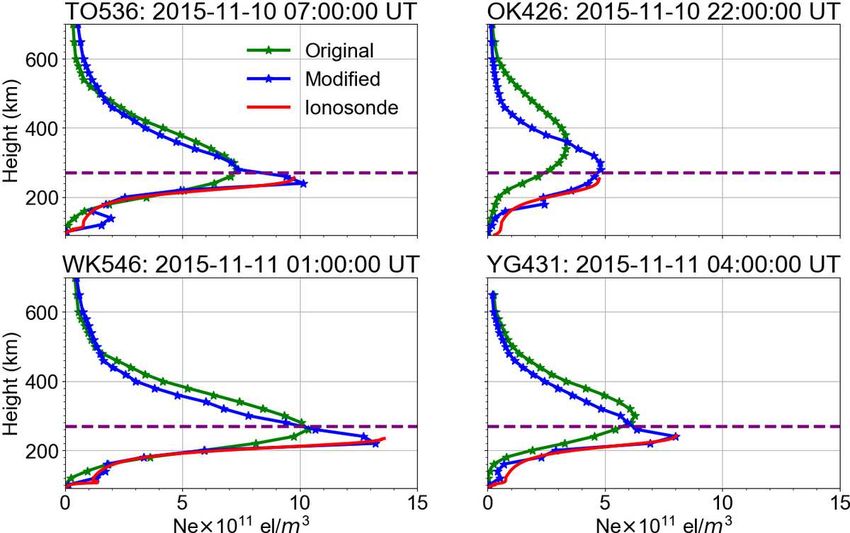
where R and B are data and background errors covariance matrices, and X b is a

vector of background log densities from the CIT solution.
 
The analysis log density X a that minimizes (4), is derived as

  ~
  ~ ~
X aj = X b + BATj −1 R + A j −1BATj −1  Y− A( X
 −1
 a
 j −1 ~  
 
 ) + A j −1[ X aj −1 − X b ]
 (5)
 ~
Where A j −1 is a Jacobian evaluated at iteration j-1. At optimal, the real densities 

 j
are computed as 10 i xa . These improvements enhanced the performance of our

tomography analysis, with the ability to track the NmF2 below the 270 km altitude

range. Figure 2 shows examples of reconstructed vertical electron density profiles at

different ionosonde locations in Japan. Refer to Figure 1 for the geographic locations.

Colours green, blue and red represent the original tomography, improved/modified

version, and ionosonde densities, respectively. In each subplot, the 270 km baseline is

illustrated with a purple horizontal dashed line. Contrary to the original tomography,

the modified version displays a distinct ability to vividly follow the measured data

both vertically and horizontally. This is effective adaptiveness, and in the sequel, we

further examine the penitential of the modified tomography under extremely chaotic

ionosphere conditions. In fact, this work is part of a pre-analysis of the modified

tomography version before advancing to a near-real-time on-line version

(https://www.enri.go.jp/cnspub/tomo3/plotting.html).

3. Analysis of reconstructions during geomagnetic storm conditions

The geomagnetic solar storm analysed occurred on St. Patrick’s day (day of year

(DOY) 076-077) in 2015 and was among the most intense storms in the 24th solar

cycle (Astafyeva et al. 2015). We reconstruct the ionosphere vertical structure during

this period (at a resolution of 15 minutes) and briefly analyse the variations in

 7

reference to the ionosphere disturbance indicator, Dst index. Specifically, the vertical

structure is analysed at ionosonde locations for easy comparison with ground

ionosonde observations. In-situ densities from the Swarm constellation and radio

occultation density profiles are also utilized to assess the reconstructed F-region

topside densities. Throughout the analysis, international reference ionosphere

(IRI-2016, Bilitza et al. 2017) model densities are also presented as a form of

reference.

3.1 Storm chronological highlights

A coronal mass ejection (CME) was observed erupting between ~ 00:30 UT -00:04

UT on DOY 074 and was predicted to encounter the Earth's magnetosphere on DOY

076. Figure 3 illustrates how the abundant energy injected into the

magnetosphere-ionosphere system perturbed the terrestrial geomagnetic field leading

to a Dst (Kp index) minimum (maximum) recording of approximately − 223 nT (8).

Kp as blue is scaled on the right and Dst as black is scaled on the left. Dashed vertical

lines indicate the main events of the storm. Both indices can be obtained from the

World Data Center for Geomagnetism, Kyoto http://wdc.kugi.kyoto‐u.ac.jp or

https://omniweb.gsfc.nasa.gov/form/dx1.html.

Before DOY 076, the geomagnetic indices Kp and Dst were relatively stable with

magnitudes below 4 and 50 nT, respectively. On DOY 076, at 04:45 UT (sudden

storm commencement, SSC), the CME hit the Earth, leading to an increase in Dst. On

the same day, at ~07:30 UT the main phase of the storm commenced and the Dst

decreased to a local minimum of ~ -80 nT. During this period the interplanetary

magnetic field (IMF) Bz component was reported to have turned Southward

(Cherniak et al. 2015). From about 9:30 UT to 12:20 UT there was a short-lived

recovery in the Dst index to ~-50 nT; expected to be due to the IMF Bz component

 8

turning Northward (Astafyeva et al. 2015). From 12:20 UT the Dst continued with a

gradually decreasing trend reaching a global minimum at ~22:00 UT on DOY 076.

The recovery phase continued through the following days with the Kp index ranging

below 6.

3.2 Analysis of reconstructions at ionosonde locations

In Figure 4 we have generated images from a time series of vertical profiles

corresponding to locations of ionosondes within the grid. The images are arranged in

accordance with increasing ionosonde geomagnetic latitude. The top, middle and

bottom panels represent the IRI-2016 model, assimilated CIT, and observations from

ionosondes, respectively. Tick labels at the top of each panel show days of the year

while those at the bottom show time in UT (the East Asian sector local time (LT) is

~9 hours ahead of UT). Preferably, IRI and reconstructed densities were converted to

frequency (MHz) for easy comparison with ionosonde measurements. The colour

scale of the frequency in each panel is given in the far right bottom corner.

In each image plate: for clarity, the altitude range is limited to the region of uttermost

interest (F-region ~200 - 600 km). Superimposed is the Dst index (ordinate axis on

the right) in order to track the response of the ionosphere during the different storm

dynamics. As indicated earlier, dashed vertical lines indicate the main events of the

storm. The horizontal dashed line at 300 km is included as a baseline to vividly track

the uplift of the plasma density. The time-altitude variation of the peak-density is

represented by the purple solid-asterisk line. In the reconstructed, and ionosonde

images, white spaces indicate periods when GPS-ground receiver ray links and

ionosonde observations did not exist or intersect that particular location. At a

 9

particular time-stamp, if there exist any data gaps within the 200-500 km altitude

range, the peak density is not determined.

Throughout the selected analysis period, at all stations, the IRI model only shows the

general diurnal variation of the F region without detailed features. This is expected

since IRI is a climatological model that represents monthly averages of terrestrial

plasma densities/frequencies (Bilitza et al. 2017). Consequently, the IRI model

performance is usually found lacking when ionosphere underlying driving

mechanisms are deviant from the general trend.

Contrary to IRI, reconstructed results reflect changes in the plasma frequency

following variations in Dst index as detailed: The onset of the storm occurred when

the East Asian sector was on the day-side. Compared to reconstructed densities on the

day before the storm (DOY 075); nearly just after the SSC, at OK426 station that is

located geomagnetically in low latitudes, there is a slight noticeable instantaneous

uplift (marked with a grey arrow) of the peak densities to altitudes above the 300 km

baseline. The uplift reduces in amplitude towards the high latitudes (not noticeable at

TO536) and is most probably due to geomagnetic storm induced eastward prompt

penetration electric fields (PPEF), which end up modifying the equatorial and low‐

latitude ionospheric phenomenology (Maruyama et al. 2004).

Approximately two hours after the SSC, there was a slight increase in F region plasma

densities (~280 - 340 km) particularly at stations located near the equatorial anomaly

(OK426 and JJ433). In addition, there was a well defined wavy modulation of the

peak density altitude at mid-latitude stations (JJ433, TO536 and IC437). The ~ 2-hour

delay falls within the time frame the traveling atmospheric disturbance (TAD) created

at high latitudes during geomagnetic storms, would take to propagate to the mid and

low latitudes (for example see the works of Shiokawa et al. 2003 and references

 10

therein). Therefore, low latitude ionisation and wavy modulation of the mid-latitude F

region could be related to an equator-wards propagating surge and plasma density

enhancements in equatorial ionization anomaly (EIA) crests, following day-side

PPEF.

By the time the East Asian sector enters the night side (~10:30 UT), there is a

short-lived recovery in the plasma frequency between 10:30 -12:30 UT. Thereafter

(~12:30 - 24:00 UT), specifically at stations located in the mid-latitudes (JJ433,

TO536 and IC437) and towards high latitudes (WK546), the plasma is uplifted to high

altitudes (~500 km), gradually falls to ~320 km, rises again to about ~380 km and

finally settles to an average altitude of ~300 km. Through this whole process, at all

stations, the initial daytime plasma enhancements decrease gradually (to values nearly

below 4 MHz), following the Dst index which hits a minimum at about 22:00 UT.

The decrease in F-region densities accompanied by descent in altitude of the peak

densities could be attributed to an equator-ward wind surge and the night-side

westward PPEF which has opposite effects (reduction in EIA ionisation) in reference

to day-side PPEF.

On the day after the storm (DOY 077), at all stations, the plasma density (frequency)

remained nearly ~60 % below the values observed on the day before the storm.

Interesting to note through this period, is the total or partial absence of data at all

ionosonde stations. From the reconstructions, it is clear that these data gaps were due

to a significant decrease in the F region plasma frequency (< 4 MHz) such that the

ionosonde could not detect the reflected echoes. This is a well-known/typical negative

ionospheric response following a major geomagnetic storm (e.g., Fuller-Rowell et al.

1994; Prölss, 1995; Tsagouri et al. 2000). A possible explanation for the intense

plasma reduction is that the sub-storm activity on DOY 076 generated a composition

 11

bulge that entered the Asian sector, and persisted through the next day (DOY 077). In

fact, Astafyeva et al. 2015 and Nava et al. 2016, analysed the thermospheric column

integrated O/N2 ratio changes measured by the GUVI (Global Ultraviolet Imager)

instrument onboard the TIMED (Thermosphere, Ionosphere, Mesosphere Energetics

and Dynamics) satellite during the same geomagnetic storm (DOY 076-078, 2015),

and found that the Asian sector had significant composition changes that could have

led to the negative ionosphere response.

Latitudinal wise, stations towards the high latitudes (WK546) exhibit the highest

reduction in plasma density. This enormous reduction in F plasma densities led to an

increase in slab thickness, which is seen to increase polewards (extending >300 km in

altitude), and most pronounced during the evening of DOY 076 and the early hours of

DOY 077. Indeed, different studies have already shown that the slab thickness is

dependent on diurnal, annual, latitudinal and storm-time variations (see Stankov and

Warnant, 2009, and references therein). In the longitudinal perspective, stations

TO536 and IC4337 that are almost on the same geomagnetic latitude (the difference is

~1°) show that the negative storm effect was greater on the Eastern side.

On the third day after the storm (DOY 078), except for OK426, all stations maintain a

slow (< 6 MHz) gradual recovery towards the normal plasma frequency values

observed during the quiet period. Nava et al. 2016 analysed the same storm and

illustrated that the recovery process lasted more than 7 days. At OK426,

reconstructions indicate that the low-latitudes had an undulating peak, accompanied

by reinforced ionisation covering altitudes ~ 200-420 km. Surprisingly, these effects

do not extend to mid-latitudes (see reconstructions at JJ433, TO536 and IC437). Nava

et al. 2016 also generated regional TEC maps corresponding to periods, before, during

and after the St. Patrick's day storm. Over the Asian sector, on the day after the storm,

 12

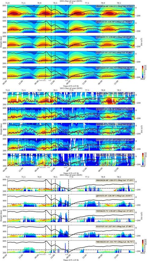
ionization was confined at low latitudes near the equator, and it almost disappeared at

middle latitudes. This ambiguous or peculiar behaviour may be related to post-storm

effects that might require further investigation (also see Kutiev et al. 2006).

GPS and ionosonde: The significance of complementing GPS with ionosonde data is

well illustrated at most stations; we can reconstruct the full extent of F region plasma

structure beyond the bottomside limitations of the ionosondes. Moreover, as noted

earlier, at points where the ionosondes failed to record any echoes due to the low

plasma electron content, our technique was still able to provide reasonable plasma

content estimations. This is a crucial result particularly for applications that utilize

trans-ionospheric HF (high frequency) signals.

3.3 Comparison with Swarm densities

In-situ densities offer a good test of accuracy since they represent a specific point in

space (ionosphere) at a particular time. The Swarm constellation consists of three

identical polar-orbiting satellites that fly at two different altitudes ≤ 460 km (Alpha (A)

and Charlie (C)) and ≤ 530 km (Bravo (B)). Each satellite has a Langmuir Probe that

facilitates the measurement of in-situ densities. Part of the Swarm density results

presented here are already presented in Ssessanga et al. 2021 (as preliminary results)

to showcase the performance of the technique. We will add more analysis plots to

cover the morning and evening sectors of the analysed period. The data used in the

analysis are Level 1b electron density measurements at a 2 Hz rate, accessible at

ftp://swarm-diss.eo.esa.int. For a further review on Swarm data see, for example,

Olsen et al. (2013).

In Figure 5, time profiles of Swarm in-situ densities (red) are plotted alongside

densities from our reconstructions (blue) and IRI model (black). Top, middle and

bottom row panels represent measurements corresponding to geographic traces

 13

(marked red on the map in the upper right corner of each subplot) of satellites A, B

and C, respectively. Each panel covers three DOYs (076, 077 and 078) during which

St. Patrick’s day storm effects were most evident. The middle sub-plots corresponding

to Swarm A and B are essentially a re-plot from Ssessanga et al. 2021, except we

added more observation data points. To match our low time resolution (15 minutes)

reconstructions with in-situ measurements, the ionosphere was assumed to remain

stationary under a period of 10 minutes. Then, all in-situ trace measurements within

this window were mapped onto the nearest altitude plane within 10 km. The vertical

dashed lines in each sub-plot indicate the start (green) and end (magenta) of grouped

traces, in which the time data gaps are less than 1-hour. Note that the x-axis in each

subplot is readjusted depending on the available traces within the day.

In all sub-plots, the agreement between the reconstructed and in-situ densities is

generally good. IRI on the other side exhibits a poor estimation of the densities. Also

noticeable is that due to differences in orbital altitudes, there is a slight difference in

the level of electron density distributions observed by satellites (A, C) and B. The

difference between in-situ and reconstructed densities is on average less than 0.2 x

1012 el/m3. This result offers confidence in the reconstructed topside F-region density

structure, which is not attainable while using ground-based instruments such as

ionosondes. A point of concern could arise from the poor density reconstructions at

the awake of profiles in time range 9:00-11:00 UT (corresponding to satellites A and

C on DOY 076 and 077). During this period Swarm A/C traces fall within or near the

equatorial latitudes. Ssessanga et al. 2021, ascribed this to a poor grid specification

over these latitudes. That is to say, the equatorial ionization anomaly region exhibits

steep latitudinal densities gradients, yet, the currently utilized grid assumes a coarse

horizontal spacing (5° × 5°) over this region (refer to Figure 1 and Saito et al. (2017;

 14

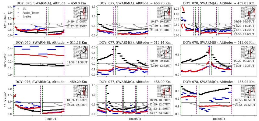
2019)), hence reconstructions would not reflect the true ionospheric state and

dynamics.

If we follow the traces of Swarm A and C, we observe that on DOY 076 when the

storm commences (~10:00-12:00 UT) the topside densities range 0.5 ~ 2 × 1012 el/

m3 . On the day that follows, during the same period, when the negative storm effects

are dominant, we observe that the densities remain nearly below 0.25 × 1012 el/m3

(~50% of the densities on DOY 076). The reduction in plasma densities is also

observed at Swarm B altitudes and is maintained throughout the late hours of DOY

077. This result is consistent with the density reductions that were observed in the

middle and bottom panels of Figure 5.

On DOY 078, when the F-region topside densities start returning to normal, the

reconstructed densities relatively track well the in-situ measurements, but with a

better performance at Swarm B altitudes. The discrepancy in performance may be

related to the altitude level; Swarm (A and C) orbit at a lower altitude (≤ 460 km) than

B, and at such altitudes the plasma densities are more likely to be influenced by

different non-linear dynamical forces during the storm period, hence making the

reconstruction acute. Certainly, the local time (~UT + 9) difference in Swarm B and

A/C observations (different ionisation levels) might also influence the results.

Nevertheless, the reconstructed densities still outperform the IRI model estimations.

3.4 Comparison with radio occultation (RO)

In Figure 6, a set of RO electron density profiles (red) from COSMIC (Constellation

Observing System for Meteorology, Climate, and Ionosphere; orbital altitude ~800

km) and GRACE (Gravity Recovery and Climate Experiment; orbital altitude ~490

km) constellations are plotted together with profiles from assimilated tomography

(blue) and IRI (black) during the analysed period. RO data are accessible in level 2

 15

format at https://cdaac-www.cosmic.ucar.edu/cdaac/. Comparison is limited to

reconstructions away from the low latitudes and above the 200 km altitude mark,

where RO density profiles are expected to have the best accuracy. That is to say, RO

density profiles are an inversion of RO total electron content (ROTEC) using the

so-called inverse Abel transform that assumes spherical symmetry in the ionosphere:

For the most part, profiles from Abel transform have good accuracy, with the

exception of the E-region (where rays have asymmetric contributions from the F

region portions of the rays), and low latitudes (where large density gradients exist,

Garcia-Fernandez et al. 2003; Wu et al. 2009; Yue et al. 2010). Rather than

comparing the RO density profiles to a specific vertical profile within the grid, the

comparison is performed at the location of tangent points (which contribute the most

density along the RO ray path) shown on the maps in the top right corner of each

subplot. Purple and green represent GRACE and COSMIC, respectively. Gaps in the

profiles indicate instances when assimilated tomography reconstructions were not

available. Fortunately, during the analysed period the GRACE constellation covered

the ~ 200-400 km range, whereas COSMIC mostly covered the topside ~ 400-700 km.

This snip view gives us a chance to nearly observe and analyse the capabilities of the

assimilated tomography in specifying the electron density field both in time and space

(horizontally and vertically).

On the DOY 075 (top left corner subplot) before the storm, both assimilated

tomography and IRI have a good estimation of the topside structure. However, on

days that follow, assimilated tomography and RO profiles show a dramatic decrease

in electron densities consequent to the geomagnetic storm. By contrast, the IRI model

maintains a high-density output, with the largest deviation from the truth in the

200-400 km altitude range. This result is important because it gives a sample of what

 16

might be expected in applications that use models to correct for ionospheric effects

during severe conditions.

Despite the variability, reconstructed profiles on average adequately track the RO

densities at all height ranges. Surprisingly, a combination of ionosonde densities and

ground-based GNSS TEC is adequate to reconstruct a reliable topside structure

(~400-700 km). Nonetheless, the noisy structure of some of the profiles motivates our

suggestion in future to integrate RO data (both TEC and electron density profiles) in

the analysis to further constrain the vertical structure.

Results presented in this study can be placed in context with previous performance

analyses of the tomography technique during the early stages of development. In this

sense, our work is a complement to studies by Seemala et al. 2014; Saito et al. 2017,

2019; Ssessanga et al. 2021, who have already analysed the tomography

reconstructions during the quiet period and found the technique to have good fidelity.

Therefore, the technique seems fairly robust in handling different ionospheric

conditions.

4. Summary

The material presented here has offered an insight into the ability of the tomography

ionosonde data assimilated technique to characterize ionosphere plasma densities

even under severe ionosphere conditions. The results clearly demonstrate that the

proposed algorithm is a good candidate for a better specification of the regional 3-D

ionosphere electron density field; reconstructed electron densities reflect changes

following the energy sink into the ionosphere system during geomagnetic storms.

Moreover, the reconstructed densities are comparable to observations covering both

bottom (ground-based ionosonde) and topside (space-borne satellites) ionosphere.

 17

Therefore, for a coherent 3-D ionosphere picture a joint use of both ground GNSS

data and bottom side ground-based ionosondes should be emphasized. However, a

more rigorous analysis should be performed to further restrain the variability in the

reconstructed vertical structure. The introduction of RO data would significantly

contribute to the structure stability. Indeed, then it would be of interest to extend our

analysis to explore and quantify the impact of the plasmasphere on the

stability/fidelity of the whole ionosphere 3-D structure.

Declarations

List of abbreviations

RO: Radio Occultation

GNSS: Global Navigation Satellite System

GPS: Global Positioning Satellite System

TEC: total electron content

STEC: Slant Total Electron Content

CIT: Computerized Ionosphere Tomography

3-D: Three-Dimensional

DOY: Day of Year

IRI: International Reference Ionosphere

CME: Coronal Mass Ejection

UT: Universal Time

LT: Local Time

IMF: Interplanetary Magnetic Field

SSC: Sudden storm Commencement

MP: Main phase

 18

PPEF: Prompt Penetration Electric Fields

TAD: Traveling Atmospheric Disturbance

EIA: Equatorial Ionization Anomaly

GUVI: Global Ultraviolet Imager

TIMED: Thermosphere, Ionosphere, Mesosphere Energetics and Dynamics

HF: High Frequency

COSMIC: Constellation Observing System for Meteorology,Climate, and Ionosphere

GRACE: Gravity Recovery and Climate Experiment

Acknowledgements

GNSS data from GEONET were provided by the Geospatial Information Authority of

Japan.

Competing interests

The authors declare that they have no competing interests.

Funding

This work is supported by the Japan Society for the Promotion of Science (JSPS)

fellowship.

Data Availability

The GNSS data can be obtained or accessed at National Geographic Information

Institute (NGII, http://www.ngii.go.kr/kor/main/main.do?rbsIdx=1) and upon request

from Geospatial Information Authority of Japan (GSI). The ionosonde data are also

accessible at http://wdc.nict.go.jp/IONO/HP2009/ISDJ/manual_txt-E.html and

ftp://ftp.ngdc.noaa.gov/ionosonde/data/. SWARM data are publicly accessible at

 19

ftp://swarm-diss.eo.esa.int. The ionospheric electron density radio occultation

observation data are downloaded from https://cdaac-www.cosmic.ucar.edu/cdaac/.

Contributions

SN conducted the research. SS and YM contributed to the algorithm design. All

authors read and approved the final manuscript.

References

Astafyeva, E., Zakharenkova I., Förster, M., (2015) Ionospheric response to the 2015

St. Patrick's Day storm: A global multi‐instrumental overview. Journal of

Geophysical Research: Space Physics, 120,10, 9023-9037.

doi:10.1002/2015JA021629

Bilitza, D., Altadill, D., Truhlik, V., Shubin, V., Galkin, I., Reinisch, B., Huang

X., (2017) International Reference Ionosphere 2016: From ionospheric climate to

real-time weather predictions. Space Weather, 15, 2, 418-429. doi:

10.1002/2016SW001593

Buonsanto, M. J., (1999) Ionospheric Storms — A Review. Space Science

Reviews, 88, 3, 563-601. doi: 10.1023/A:1005107532631

Bust, G. S., Coco, D., Makela, J. J., (2000) Combined Ionospheric Campaign 1:

Ionospheric tomography and GPS total electron count (TEC) depletions. Geophysical

research letters, 27, 18, 2849-2852. doi: 10.1029/2000GL000053

 20

Bust, G. S., Mitchell, C. N., (2008) History, current state, and future directions of

ionospheric imaging. Reviews of Geophysics, 46, RG1003. doi:

10.1029/2006RG000212

Cannon, P., Angling, M., Barclay, L., Curry, C., Dyer, C., Edwards, R., Greene, G.,

Hapgood, M., Horne, R.B., Jackson, D., Mitchell, C.N., (2013) Extreme space

weather: impacts on engineered systems and infrastructure. Royal Academy of

Engineering. doi: 1-903496-95-0

Chen, C. H., Saito,A., Lin, C. H., Yamamoto, M., Suzuki, S., Seemala, G. K.,

(2016) Medium‐scale traveling ionospheric disturbances by three‐dimensional

ionospheric GPS tomography. Earth Planets and Space, 68, 32. doi:

10.1186/s40623-016-0412-6

Cherniak, I., Zakharenkova, I., Redmon, R. J., (2015) Dynamics of the high-latitude

ionospheric irregularities during the 17 March 2015 St. Patrick's Day storm:

Ground-based GPS measurements. Space Weather, 13, 9, 585-597. doi:

10.1002/2015SW001237

Eastwood, J. P., Biffis, E., Hapgood, M. A., Green, L., Bisi, M. M., Bentley, R. D.,

Wicks, R., McKinnell, L. A., Gibbs, M., Burnett, C., (2017) The economic impact of

space weather: Where do we stand?. Risk Analysis, 37, 2, 206-218.

doi:10.1111/risa.12765

Garcia-Fernandez, M., Hernandez-Pajares, M., Juan, M., Sanz, J., (2003)

 21

Improvement of ionospheric electron density estimation with GPSMET

occultations using Abel inversion and VTEC information, Journal of Geophysical

Research: Space Physics, 108, A9, 1338. doi: 10.1029/2003JA009952

Fremouw, E. J., Secan, J. A., Howe, B.M., (1992) Application of stochastic inverse

theory to ionospheric tomography. Radio Science, 27, 5, 721-732. doi:

10.1029/92RS00515

Fuller-Rowell, T., Codrescu, M., Moffffett, R., Quegan, S., (1994) Response of the

thermosphere and ionosphere to geomagnetic storms. Journal of Geophysical

Research: Space Physics, 99, A3, 3893-3914. doi:10.1029/93JA02015

Howe, B. M., Runciman K., Secan, J. A., (1998) Tomography of the ionosphere:

Four‐dimensional simulations, Radio Science, 33, 1, 109-128. doi:

10.1029/97RS02615

Jakowski, N., Béniguel, Y., De Franceschi, G., Pajares, M. H., Jacobsen, K. S.,

Stanislawska, I., Tomasik, L., Warnant, R., Wautelet, G., (2012) Monitoring, tracking

and forecasting ionospheric perturbations using GNSS techniques. Journal of Space

Weather and Space Climate, 2, A22. doi: 10.1051/swsc/2012022

Jakowski, N., Mayer, C., Hoque, M. M., Wilken, V., (2011) Total electron content

models and their use in ionosphere monitoring. Radio Science, 46, RS0D18. doi:

10.1029/2010RS004620

 22

Kelly, M.A., Comberiate, J.M., Miller, E.S., Paxton, L.J., (2014) Progress toward

forecasting of space weather effects on UHF SATCOM after Operation

Anaconda. Space Weather, 12, 10, 601-611. doi: 10.1002/2014SW001081

Kutiev, I., Otsuka, Y., Saito, A., Watanabe, S., (2006) GPS observations of post-storm

TEC enhancements at low latitudes. Earth, planets and space, 58, 11, 1479-1486.

doi:10.1186/BF03352647

Ma, X. F., Maruyama, T., Ma, G., Takeda, T., (2005) Three‐dimensional ionospheric

tomography using observation data of GPS ground receivers and ionosonde by neural

network. Journal of Geophysical Research: Space Physics, 110, A5. doi:

10.1029/2004JA010797

Ma, G., Maruyama, T., (2003) Derivation of TEC and estimation of instrumental

biases from GEONET in Japan. Annales Geophysicae, 21, 10, 2083-2093. doi:

10.5194/angeo-21-2083-2003

Maruyama, T., Ma, G., Nakamura, M., (2004) Signature of TEC storm on 6

November 2001 derived from dense GPS receiver network and ionosonde chain over

Japan. Journal of Geophysical Research, 109, A10302. doi: 10.1029/2004JA010451

Mitchell, C. N., Spencer, P. S., (2003) A three‐dimensional time‐dependent algorithm

for ionospheric imaging using GPS. Annales Geophysicae, 46, 4, 687-696. doi:

10.4401/ag-4373

 23

Nava, B., Coisson, P., Radicella, S. M., (2008) A new version of the NeQuick

ionosphere electron density model. Journal of Atmospheric and Solar-Terrestrial

Physics, 70, 15, 1856-1862. doi: 10.1016/j.jastp.2008.01.015

Nava, B., Rodríguez‐Zuluaga, J., Alazo‐Cuartas, K., Kashcheyev, A., Migoya‐Orué,

Y., Radicella, S. M., Amory‐Mazaudier, C., Fleury, R., (2016) Middle‐and low‐

latitude ionosphere response to 2015 St. Patrick's Day geomagnetic storm. Journal of

Geophysical Research: Space Physics, 121, 4, 3421-3438. doi:

10.1002/2015JA022299

Ohashi, M., Hattori, T., Kubo, Y., Sugimoto, S., (2013) Multi-layer ionospheric

VTEC estimation for GNSS positioning. Transactions of The Institute of Systems,

Control and Information Engineers, 26, 1, 16-24.

Okoh, D. I., McKinnell, L. ‐A., Cilliers, P. J., (2010), Developing an ionospheric map

for South Africa. Annales Geophysicae, 28, 7, 1431-1439. doi: 10.5194/angeo‐28‐

1431‐2010

Olsen, N., Friis‐Christensen, E., Floberghagen, R., Alken, P., Beggan, C. D., Chulliat,

A., Doornbos, E., da Encarnao, J. T., Hamilton, B., Hulot, G., van den IJssel,

J., Kuvshinov, A., Lesur, V., Lhr, H., Macmillan, S., Maus, S., Noja, M., Olsen, P. E.

H., Park, J., Plank, G., Pthe, C., Rauberg, J., Ritter, P., Rother, M., Sabaka, T.

J., Schachtschneider, R., Sirol, O., Stolle, C., Thbault, E., Thomson, AlanW.

P., Tffner‐Clausen, L., Velmsk, J., Vigneron, P., Visser, (2013) The Swarm Satellite

 24

Constellation Application and Research Facility (SCARF) and Swarm data

products. Earth, Planets and Space, 65, 11, 1189-1200. doi: 10.5047/eps.2013.07.001

Otsuka, Y., Ogawa, T., Saito, A., Tsugawa, T., Fukao, S., Miyazaki, S., (2002) A new

technique for mapping of total electron content using GPS network in Japan. Earth,

planets and space, 54, 1, 63-70. doi: 10.1186/BF03352422

Prölss, G. W., (1995) Ionospheric F‐region storms. In Handbook of Atmospheric

Electrodynamics, Volland, H (ed), 2nd edn, CRC Press, Boca Raton, Florida.

Raymund, T. D., Franke, S. J., Yeh, K. C., (1994) Ionospheric tomography: its

limitations and reconstruction methods. Journal of atmospheric and terrestrial physics,

56, 5, 637-657. doi: 10.1016/0021-9169(94)90104-X

Rius, A., Ruffini, G., Cucurull, L., (1997) Improving the vertical resolution of

ionospheric tomography with GPS occultations. Geophysical Research Letters, 24,18,

2291-2294. doi: 10.1029/97GL52283

Rovira-Garcia, A., Ibanez-Segura, D., Orus-Perez, R., Juan, J. M., Sanz, J.,

Gonzalez-Casado, G., (2020) Assessing the quality of ionospheric models through

GNSS positioning error: methodology and results. Gps solutions, 24,1, 1-12. doi:

10.1007/s10291-019-0918-z

 25

Schmidt, M., Bilitza, D., Shum, C., Zeilhofer, C., (2008) Regional 4D modeling of the

ionospheric electron density. Advances in Space Research, 42, 4, 782-790. doi:

10.1016/j.asr.2007.02.050

Saito, A., Miyazaki, S., Fukao, S., (1998) High resolution mapping of TEC

perturbations with the GSI GPS network over Japan. Geophysical Research Letters,

25, 16, 3079-3082. doi: 10.1029/98GL52361

Saito, S., Suzuki, S., Yamamoto, M., Saito, A., Chen, C. H., (2017) Real‐time

ionosphere monitoring by three‐dimensional tomography over Japan. Navigation:

Journal of the Institute of Navigation 64, 4, 495-504. doi: 10.1002/navi.213

Saito, S., Yamamoto, M., Saito, A., Chen, C. H., (2019) Real-time 3-D Ionospheric

Tomography and Its Validation by the MU Radar. In 2019 URSI Asia-Pacific Radio

Science Conference (AP-RASC). IEEE (pp. 1-1). doi:

10.23919/URSIAP-RASC.2019.8738382

Seemala, G. K., Yamamoto, M., Saito A., Chen, C. -H., (2014) Three-dimensional

GPS ionospheric tomography over Japan using constrained least squares. Journal of

Geophysical Research: Space Physics, 119, 4, 3044-3052. doi:

10.1002/2013JA019582

Shiokawa, K., Otsuka, Y., Ogawa, T., Kawamura, S., Yamamoto, M., Fukao, S.,

Nakamura, T., Tsuda, T., Balan, N., Igarashi, K., Lu, G., (2003) Thermospheric wind

 26

during a storm‐time large‐scale traveling ionospheric disturbance. Journal of

Geophysical Research: Space Physics, 108, A12, 1423. doi: 10.1029/2003JA010001

Ssessanga, N., Yamamoto, M., Saito, S., Saito, A., Nishioka M., (2021)

Complementing regional ground GNSS-STEC computerized ionospheric tomography

(CIT) with ionosonde data assimilation, GPS solutions (under review,

GPSS-D-20-00186)

Ssessanga, N., Kim, Y. H., Kim, E., (2015) Vertical structure of medium‐scale

traveling ionospheric disturbances (MSTIDs). Geophysical Research Letters, 42, 21,

9156-9165. doi:10.1002/2015GL066093

Stankov, S. M, Warnant, R., (2009) Ionospheric slab thickness-analysis, modelling

and monitoring. Advances in Space Research, 44, 11, 1295-1303. doi:

10.1016/j.asr.2009.07.010

Tsagouri, I., Belehaki, A., Moraitis, G., and Mavromichalaki, H., (2000) Positive and

negative ionospheric disturbances at middle latitudes during geomagnetic storms.

Geophysical Research Letters, 27, 21, 3579-3582. doi: 10.1029/2000GL003743

Tsai, L. ‐C., Liu, C., Tsai, W., Liu, C., (2002) Tomographic imaging of the

ionosphere using the GPS/MET and NNSS data. Journal of Atmospheric and

Solar-terrestrial Physics, 64, 18, 2003-2011. doi: 10.1016/S1364-6826(02)00218-3

 27

Wu, X., Hu, X., Gong, X., Zhang, X., Wang, X., (2009), Analysis of the inversion

error of ionospheric occultation. GPS Solutions, 13, 3, 231- 239. doi:

10.1007/s10291‐008‐0116‐x

Yasyukevich, Y., Astafyeva, E., Padokhin, A., Ivanova, V., Syrovatskii, S., Podlesnyi,

A., (2018) The 6 September 2017 X‐class solar flares and their impacts on the

ionosphere, GNSS, and HF radio wave propagation. Space Weather, 16, 8, 1013-1027.

doi: 10.1029/2018SW001932

Yeh, K. C., Raymund, T. D., (1991) Limitations of ionospheric imaging by

tomography. Radio Science, 26 , 6, 1361-1380. doi: 10.1029/91RS01873

Yue, X., Schreiner, W. S., Lei, J., Sokolovskiy, S. V., Rocken, C., Hunt, D. C., Kuo,

Y.‐H., (2010) Error analysis of Abel retrieved electron density profiles from radio‐

occultation measurements. Annales Geophysicae, 28, 1, 217- 222.

doi: 10.5194/angeo‐28‐217‐2010

Figure Legends

Figure 1: Image obtained from the works of Ssessanga et al. 2021: A network of

GNSS receivers (blue asterisks) and ionosonde stations (solid red stars) used in the

analysis. Horizontal boundaries of the different sub-grid regions that compose the

overall grid used in computation are marked by solid dashed lines. The sub-grid

resolution decreases with increasing distance away from the dense network.

 28

Figure 2: Examples density profiles reconstructed density profiles at different

ionosonde locations in Japan. The time stamps are indicated at the top of each subplot.

The original tomography densities without the assimilation complexity are shown in

green. Eminent is the robustness of the modified version (blue) to track the ionosonde

measured (red) densities below the 270 km altitude range (purple line).

Figure 3: Variation of Kp and Dst indices during the 2015 St. Patrick's day

geomagnetic storm. Tick labels on top and bottom represent day of the year (DOY)

and Time in UT (~LT-9 hours), respectively. The Sudden storm Commencement

(SSC) occurred at ~04:45 on DOY 076. The main phase (MP) of the storm started at

~06:30 UT and continued until ~22:00 UT when Dst hit a minimum ~ -223 nT.

During the MP the Kp rose to a maximum of ~8. The recovery phase continued

through the following days.

Figure 4: Ionosphere vertical structure at 5 ionosonde locations within the grid,

during the 2015 St. Patrick’s Day solar storm. Top, middle and bottom panels

represent IRI-2016, reconstructed, and ionosonde observations, receptively. Stations

in each panel are arranged in ascending geomagnetic latitude. Tick labels on top and

bottom of each panel represent day of the year (DOY) and Time in UT (~LT-9 hours),

respectively. Scaled on the right of each image is Dst index, represented by the solid

black line. Vertical dashed lines indicate the main events of the storm. In the IRI and

reconstructed images, the purple solid-asterisk line shows the time variation of the

hmF2 parameter at that ionosonde location.

 29

Figure 5: A plot of time-density profiles following the Swarm satellite orbital path

(shown as red traces on the map in the upper right corner of each sub-plot); black,

blue and red represent IRI, reconstructed and Swarm in-situ densities, respectively.

Vertical dashed lines show the start (green) and end (magenta) of grouped together

traces, with time data gaps less than 1 hour. Column-wise: Top, middle and bottom

panels correspond to Swarm Alpha (A), Charlie (C) and Bravo (B), respectively.

Row-wise: Right, middle and left sub-plots correspond to day of year 076, 077 and

078, respectively, when storm effects were eminent. Note that the x-axis depends on

the number of available traces.

Figure 6: Comparison of radio occultation (RO) to IRI model (black) /reconstructed

(blue) density profiles during the 2015 St Patrick's day geomagnetic storm.

Comparison is performed along the trace of RO tangent points shown on maps in the

upper right corner of each subplot (purple: GRACE, green: COSMIC). DOY 076 is

not presented because the data points were few. Also, we limit the analysis to regions

where RO density profiles have good accuracy (away from the low latitudes and

altitudes above 200 km).

 30

Figures

Figure 1

Image obtained from the works of Ssessanga et al. 2021: A network of GNSS receivers (blue asterisks)
and ionosonde stations (solid red stars) used in the analysis. Horizontal boundaries of the different sub-
grid regions that compose the overall grid used in computation are marked by solid dashed lines. The
sub-grid resolution decreases with increasing distance away from the dense network. Note: The
designations employed and the presentation of the material on this map do not imply the expression of
any opinion whatsoever on the part of Research Square concerning the legal status of any country,

territory, city or area or of its authorities, or concerning the delimitation of its frontiers or boundaries. This
map has been provided by the authors.

Figure 2

Examples density pro les reconstructed density pro les at different ionosonde locations in Japan. The
time stamps are indicated at the top of each subplot. The original tomography densities without the
assimilation complexity are shown in green. Eminent is the robustness of the modi ed version (blue) to
track the ionosonde measured (red) densities below the 270 km altitude range (purple line).

Figure 3

Variation of Kp and Dst indices during the 2015 St. Patrick's day geomagnetic storm. Tick labels on top
and bottom represent day of the year (DOY) and Time in UT (~LT-9 hours), respectively. The Sudden
storm Commencement (SSC) occurred at ~04:45 on DOY 076. The main phase (MP) of the storm started
at ~06:30 UT and continued until ~22:00 UT when Dst hit a minimum ~ -223 nT. During the MP the Kp
rose to a maximum of ~8. The recovery phase continued through the following days.

Figure 4

Ionosphere vertical structure at 5 ionosonde locations within the grid, during the 2015 St. Patrick’s Day
solar storm. Top, middle and bottom panels represent IRI-2016, reconstructed, and ionosonde
observations, receptively. Stations in each panel are arranged in ascending geomagnetic latitude. Tick
labels on top and bottom of each panel represent day of the year (DOY) and Time in UT (~LT-9 hours),
respectively. Scaled on the right of each image is Dst index, represented by the solid black line. Vertical

dashed lines indicate the main events of the storm. In the IRI and reconstructed images, the purple solid-
asterisk line shows the time variation of the hmF2 parameter at that ionosonde location.

Figure 5

A plot of time-density pro les following the Swarm satellite orbital path (shown as red traces on the map
in the upper right corner of each sub-plot); black, blue and red represent IRI, reconstructed and Swarm in-
situ densities, respectively. Vertical dashed lines show the start (green) and end (magenta) of grouped
together traces, with time data gaps less than 1 hour. Column-wise: Top, middle and bottom panels
correspond to Swarm Alpha (A), Charlie (C) and Bravo (B), respectively. Row-wise: Right, middle and left
sub-plots correspond to day of year 076, 077 and 078, respectively, when storm effects were eminent.
Note that the x-axis depends on the number of available traces. Note: The designations employed and the
presentation of the material on this map do not imply the expression of any opinion whatsoever on the
part of Research Square concerning the legal status of any country, territory, city or area or of its
authorities, or concerning the delimitation of its frontiers or boundaries. This map has been provided by
the authors.

Figure 6

Comparison of radio occultation (RO) to IRI model (black) /reconstructed (blue) density pro les during
the 2015 St Patrick's day geomagnetic storm. Comparison is performed along the trace of RO tangent
points shown on maps in the upper right corner of each subplot (purple: GRACE, green: COSMIC). DOY
076 is not presented because the data points were few. Also, we limit the analysis to regions where RO
density pro les have good accuracy (away from the low latitudes and altitudes above 200 km). Note: The
designations employed and the presentation of the material on this map do not imply the expression of
any opinion whatsoever on the part of Research Square concerning the legal status of any country,
territory, city or area or of its authorities, or concerning the delimitation of its frontiers or boundaries. This
map has been provided by the authors.

Supplementary Files
This is a list of supplementary les associated with this preprint. Click to download.

 PaperAbstractpic.png