Altimetry on the second military survey maps in the territories of Bohemia, Moravia and Silesia
←
→
Page content transcription
If your browser does not render page correctly, please read the page content below
e-Perimetron, Vol. 5, No. 3, 2010 [144-159] www.e-perimetron.org | ISSN 1790-3769
Martina Vichrova∗, Vaclav Cada∗∗
Altimetry on the second military survey maps in the territories
of Bohemia, Moravia and Silesia
Keywords: Altimetry; Second Military Survey; Bohemia; Moravia; Silesia.
Summary: The Second Military Survey in the territories of the former Austrian-Hungarian
Monarchy was done between 1806 and 1869. Its purpose was to remove the defects of the First
Military Survey including gross position errors and cartographic representation defects of ob-
jects in maps, and to contribute to a well-arranged map for the entire monarchy. In the territo-
ries where the cadastral survey was completed (Bohemia, Moravia, Silesia, etc.) the outcomes
were exploited for the military survey. Reduced and generalised planimetric content from the
cadastral maps and cadastral triangulation was used to outline the planimetric content of the
Second Military Survey. This assured an improved positional accuracy and better work econ-
omy. The territory of Bohemia was surveyed between 1842 and 1853 (267 handwritten colour
sections 1:28 800), Moravia and Silesia between 1836 and 1840 (146 handwritten colour sec-
tions 1:28 800). Currently, the map originals are stored in the Vienna Military archive depart-
ment of the Austrian State Archives.
The aim of this contribution is to describe the methodology of altimetry and determination of
heights displayed on the Second Military Survey maps of Bohemia, Moravia and Silesia. The
accuracy of the elevations has been analysed. Attention is paid to the portrayal of altimetry on
the maps.
The Second Military Survey (Franziszeische Landesaufnahme) 1806 – 1869
The original concept of the Second Military Survey
The Second Military Survey was launched on 2nd April 1806 by a decree of Emperor Francis II1
(Hofstätter 1989: 61). In the same year the Emperor also authorized a proposal by general
A. Mayer von Heldensfeld2, head of general quartermaster staff (Generalquartiermeisterstab), to
establish the military triangulation (Boguszak and Cisar 1961: 14), called the astronomical-
geodetical network, for the whole territory of the Austrian monarchy as a reference coordinate
frame of the Second Military Survey. The Topographic Institute in Vienna initiated the first
measurements in 1806 and triangulation works proceeded in difficult conditions with a small
number of officers.
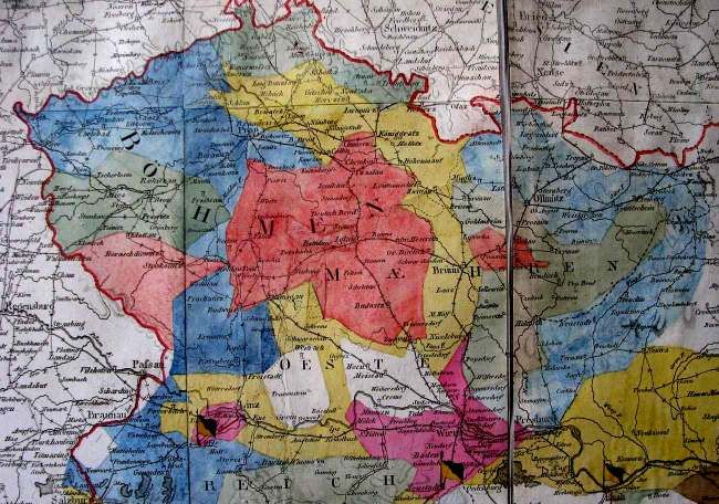
The military triangulation was completed for Bohemia, Moravia, and Silesia by 1811 (Fig. 1). The
coordinates of the trigonometric points were probably used for the revision of the topographic
survey in Bohemia between 1812 and 1819.
∗
MSc. Martina Vichrova, University of West Bohemia in Pilsen, Univerzitni 22, 306 14 Pilsen, Czech Republic,
[vichrova@kma.zcu.cz]
∗∗
Assoc. Prof. Vaclav Cada, University of West Bohemia in Pilsen, Univerzitni 22, 306 14 Pilsen, Czech Repub-
lic [cada@kma.zcu.cz]
1
Emperor Francis (*1768 – †1835) was the first Roman (Francis the I.) and thus the second Austrian emperor
(Francis the II.). He dominated in years 1792 – 1835.
2
Anton Freiherr Mayer von Heldensfeld (*1765 – †1842) Field-Marshal of Austrian army (Nischer 1925: 108).
[144]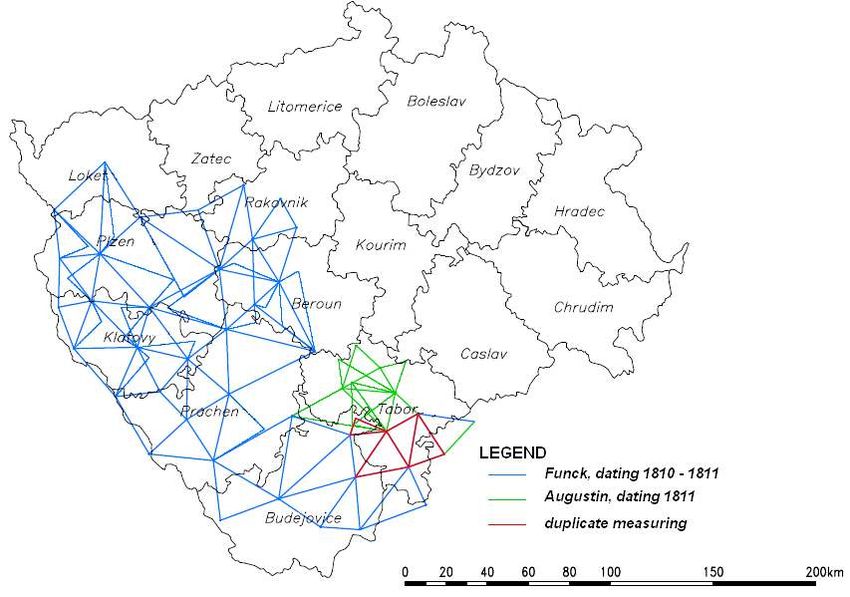
e-Perimetron, Vol. 5, No. 3, 2010 [144-159]                                              www.e-perimetron.org | ISSN 1790-3769

The complete network of the military triangulation was originally intended as a uniform coordi-
nate reference system (St. Stephen), in order to create a continuous display of the whole monarchy
in the uniform layout of map sheets. Marshal Fallon, Marshal Maurich, Marshal Mertz, Lieutenant
Kielmann and Lieutenant Schweiger took part in the majority of measurements.
The original plan was to display the whole monarchy in the Cassini-Soldner transversal cylindri-
cal projection with the central meridian passing through the St. Stephen trigonometric station. The
map sheets in the so-called older section division formed a plane network of rectangles in scale
1:28 800 with sizes of 24 x 16 Viennese inches (63 x 42 cm), parallel with coordinate axes, dis-
playing an area of 2,4 x 1,6 Austrian mile (18 x 12 km) (Kuchar 1967: 82). The sections were in-
dicated from west to east by capital letters R, Q, ….A, then by roman numerals I, II, …LXIV. The
rows were indicated from north to south by 16, 17, …102. Selected map sheets around large cit-
ies, strategically important objects, military objects and exercising grounds were represented in
scale 1:14 400.

 Figure 1: Military triangulation built in the former territory of Bohemia, Moravia and Silesia between 1806 and 1811. The
      territory triangulated in 1806 – pink, 1807 – yellow, 1808 – blue, 1810 – dark green, 1811 – red, (Arbeiten des
                                           k. k. Generalquartiermeisterstabs… 1850).

The plane table method was used for the detailed topographic survey. The planimetric objects
were included in the military triangulation network by graphical intersections, pacing or distance
estimation.

                                                          [145]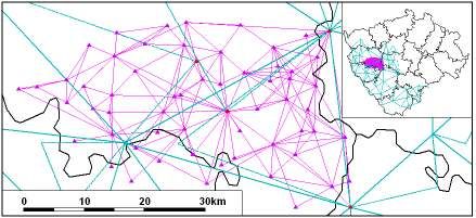
e-Perimetron, Vol. 5, No. 3, 2010 [144-159]                                     www.e-perimetron.org | ISSN 1790-3769

                                 The modified concept of the Second Military Survey

In some territories (e.g. Bohemia, Moravia, Silesia, Dalmatia, Carinthia) the cadastre survey was
already finished or in progress. This allowed a modified approach for the Military Survey by us-
ing actual results of the cadastre survey. This combination was also used for the general topog-
raphic and administrative maps of individual territories of the monarchy. The modification ap-
plied to both horizontal control and cartographical foundations. It also affected the process of sur-
veying.
The trigonometric network was established by the triangulation office of i.r. (imperial royal) Gen-
eral Staff (k.k. Generalstab). Between 1807 and 1840 the triangulation network was established
exclusively by military officers. Later, civil topographers cooperated as well. The network was
constructed in distinct steps, beginning with first order points, subsequently densified later until
the fourth order. The detailed surveying works began when the triangulation had been completed.
The first order network (Grosses Netz) was established in Bohemia between 1824 and 1825, and
1827 and 1840, and in Moravia between 1821 and 1826 (Cada 2005: 36). The densification to
second and third order (Kleines Netz) depended on the progress of the surveying. The second and
the third order networks were established in Bohemia between 1825 and 1840, and in Moravia
between 1822 and 1829 (Cada 2005: 36). All the networks were completed in 1858.
According to Boguszak and Cisar (1961: 16) and Cada (2005: 37) the coordinates for Bohemia
were given in a plane coordinate system with the origin at the trigonometric station Gusterberg.
For Moravia and Silesia the origin was at the trigonometric station St. Stephen in Vienna. The
networks from the first to the third order in Bohemia (51 953 km2) contained 2 623 trigonometric
points. Permanent marking was made between 1845 and 1850, when only 2 234 points were lo-
cated and monumented. In Moravia and Silesia (27 375 km2) there were 1 069 points between
1850 and 1852, but only 833 were monumented. The height above sea level (Adriatic system) of
the trigonometric points was determined in Viennese fathoms with two decimal positions. More
information about the geodetic control and its use for the Second Military Survey can be found in
Cada and Vichrova (2009).
The Cassini-Soldner projection was also used for the cadastre survey. The central meridian was
chosen in the centre of a territory and passed through a significant station of the trigonometric
network (Gusterberg, St. Stephen). The reasons for using more than one reference point was the
practical task of producing maps for several administrative regions and the need to cover the
whole monarchy with cadastral maps. Also, an unfavourable longitudinal distortion in parallels
existed in the border regions.
The usage of geodetic and cartographic controls for cadastre survey and generalized cadastral
planimetry is the major feature of the modified concept of the Second Military Survey. In conse-
quence these changes invocated another layout of the map. The new map sheets of the Second
Military Survey were derived from the map sheets of stable cadastre, i.e. a division of a plane co-
ordinate system with parallels to the coordinate axes. The new map sections (2 x 2 Austrian miles
= 800 x 800 fathoms) were scaled 1:28 800 to 20 x 20 Viennese inches, i.e. 52,7 x 52,7 cm (Bo-
guszak and Cisar 1961: 16; Kuchar 1967: 85). One map section of the Second Military Survey
displayed an area of four fundamental sheets of the stable cadastre. The columns (Colonne) paral-
lel to the X axis were numbered with Roman numerals in the direction from east (O – ostliche
Colonne) to west (W – westliche Colonne). The rows (Schichte) parallel to the Y axis were num-
bered with Arabic numerals from north to south (Boguszak and Cisar 1961: 16; Kuchar
1967: 84 – 85).

                                                       [146]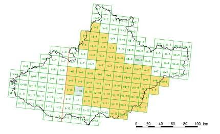
e-Perimetron, Vol. 5, No. 3, 2010 [144-159]                                             www.e-perimetron.org | ISSN 1790-3769

In territories where the cadastral survey was already finished or in progress, the planimetric con-
tents of cadastral maps in scale 1:2 880 were used. They were pantographically reduced and sim-
plified to the scale 1:28 800. The short time between the cadastral and topographic surveys al-
lowed the use of most of the planimetry. The topographer adjusted only the planimetry according
to the military legend and surveyed the terrain relief and some new objects that were not displayed
in cadastral maps.
Using the cadastral planimetry significantly accelerated and rationalised the topographic works. In
such territories, one topographer and an assistant completed 3 sections of the new map sheets each
year. This is equal to 12 square Austrian miles each year or 690 km2. The original concept (with-
out using the planimetry of cadastral maps) planned for only 4 – 6 square Austrian miles each
year (230 – 345 km2). The acquisition costs of mapping of one square Austrian mile decreased
from 250 to 120 Gulden (Kuchar 1967: 84). The main differences between the original and the
modified concepts are shown in Table 1.
Original map sections in scale 1:28 800 for Bohemia (267 handwritten colour sections 1:28 800),
Moravia and Silesia (146 handwritten colour sections 1:28 800) are kept in the map collection of
the Austrian State Archives – Military Archive in Vienna (Österreichisches Staatsarchiv –
 Kriegsarchiv Wien).

          Comparative characteristics                  Original concept                 Modified concept

        Triangulation                                       military                         cadastral

        System of coordinates                             St. Stephen                 St. Stephen, Gusterberg

        Section indexing                                    original                         modified

        Size of one map section                     24´´ x 16´´ (63 x 42 cm)       20´´ x 20´´ (52,7 x 52,7 cm)

        Displayed territory                               18 x 12 km                        15 x 15 km
        Area of territory displayed on one
                                                          221,0 km2                         230,2 km2
        map sheet
                                                Topographic survey with a meas-
        Surveying method                                                            Use of cadastral planimetry
                                                         uring table

                                                 All sections without regard to   Only territory within provincial
        Map drawing
                                                       provincial borders                     borders

            Table.1 Major differences between original and modified concepts for Bohemia, Moravia and Silesia.

                                              Portrayal of altimetry on maps

The altimetry on the maps of the Second Military Survey is portrayed according to the legend
shown in Muster-Blätter… (1831 – 1840) by Lehmann hachures and spot heights. The hachures
portray not only the direction of the maximum gradient but also the slope of the terrain. The slope
is portrayed by functionally dependent length and thickness of the hachures and distances between
them according to the precise scale (Fig. 2). The map legend includes type models of the elemen-
tary landforms. Each of these model landforms is displayed by contours with inclined cuts in im-
portant profiles (Fig. 3). From all the cartographic map symbols shown in Muster-
Blätter… (1831 – 1840) the Feature Catalogue of the Second Military Survey was produced. The
whole catalogue is present and described in detail in Vichrova (2005). A digital version of the
catalogue can be found at: http://home.zcu.cz/~vichrova/clanky/Katalog_objektu_VII.pdf.

                                                             [147]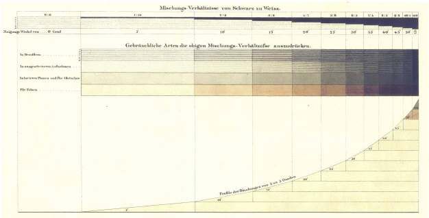
e-Perimetron, Vol. 5, No. 3, 2010 [144-159]                                                 www.e-perimetron.org | ISSN 1790-3769

                    Figure 2: Scale for portrayal of the slope of the terrain. (Muster-Blätter… 1831 – 1840).

Figure 3 depicts a model example of one of the landforms present in the feature catalogue. This
includes mountains, rocks and mountain glaciers, plains, highlands, Alpine-type mountains,
mountains with permanent snow cover and karst mountains. The example depicts a gully. The
description of the landform and geographical names are not present but these are included in the
final map sheets of the Second Military Survey. The cuts depicting the character of the terrain are
shown on the model example.

Figure 3: Landform – gully: portrayal using hachures and appropriate geometric model with depicted cutting planes and pro-
                                           files (Muster-Blätter… 1831 – 1840).

The representation of the terrain on maps using hachure gives a true plastic image of the terrain,
as well as objective and visual information about the permeability of the area. The disadvantage of
this method is a high graphical load of the map sheet in comparison with other symbols on the
map.
The representation of the landforms on the maps of the Second Military Survey was accomplished
by spot heights chosen mostly from geodetic control. The heights on the map sheets of Bohemia,
Moravia and Silesia are produced according to the modified technology in units of Viennese fath-
oms with an accuracy of two decimal points (Fig. 4). No spot heights were found on the map
sheets in the area of South Bohemia (Vitorazsko) which were produced according to the original
technology.
The following section of the paper is focused mainly on the methods of determination of the spot
heights and analysis of their accuracy.

                                                             [148]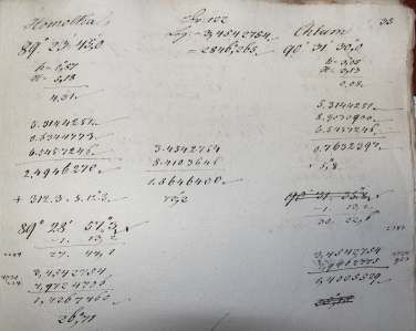
e-Perimetron, Vol. 5, No. 3, 2010 [144-159]                                                www.e-perimetron.org | ISSN 1790-3769

                              Figure 4: An example of the depiction of the spot height on the map.

                         Available sources and methodology of height determination

                       Determination of heights from military triangulation measurements

The building of the military triangulation of the Austrian Monarchy began in 1806. After sample
measurements and setting the methodology for processing of the measured data the “Instruction
für die bey der k. k. österreichischen Landes-Vermessung angestellten Herren Officiere” was pub-
lished in 1810 (Binnenthal 1810). The methodology should have ensured a unified approach in
building the triangulation network and also the processing of measured data. The military triangu-
lation in the former territory of Bohemia, Moravia and Silesia was built between 1806 and 1811
(Fig. 1).
The triangulation record also contains calculation records (Funck 1810 – 1811; Augustin 1811)
with determined heights of trigonometric points including their differences in elevation. The cal-
culation records contain measured values including height of the standpoint, height of the target
and measured zenithal distance; values taken from other calculation records including logarithm
of the length or length, coefficient of refraction; and calculated values including zenithal length
reduction, differences in elevation, elevation of trigonometric points and targeted points located
on them.
The determination of heights was done by trigonometric measuring of zenithal lengths on targeted
points. The distance between the targeted points was several tens of kilometres. The zenithal
lengths were reduced to the elevation of the standpoint and also to the targeted point. Differences
in elevation between trigonometric points were calculated from the reduced zenithal lengths and
the lengths of the sides. Then the height above sea level of the targeted point was calculated from
a minimum of two various points with previously determined heights. The final height of the de-
termining point was set by arithmetic mean. If the height of the targeted point was also measured
then the height above sea level of the natural terrain at the trigonometric point was calculated.
The calculation network and the heights of the trigonometric points were reconstructed from the
calculation records (Funck 1810 – 1811; Augustin 1811) for the territories that according to the
administrative division from the years between 1751 and 1842 encompassed the whole territory of
the Pilsen, Klatovy and Prachen regions, and for parts of the Loket, Zatec, Beroun, Tabor and
Budejovice regions. The location of the territories is shown in Figure 5. The network built be-
tween 1810 and 1811 by Hejtmann Funck is blue. The network built in 1811 by Hejtmann Au-
gustin is green. The network shown in red is a part of the trigonometric network that was meas-
ured twice by both these surveyors.

                                                             [149]
e-Perimetron, Vol. 5, No. 3, 2010 [144-159] www.e-perimetron.org | ISSN 1790-3769
Figure 5: Calculation network for determination of heights of trigonometric points reconstructed according to Funck (1810 –
1811) and Augustin (1811). The background layer represents administrative division from the years between 1751 – 1842.
From the differences in elevation of individual sides the height misclosures were calculated for
triangles of the calculation network: u= ∆h1 + ∆h2 + ∆h3, where ∆h1, ∆h2 and ∆h3 are differences
in elevation between the vertices of the triangle. Then the average value of the height misclosure
was set u :
n
∑u
i =1
i
u=
n
In this calculation n is the number of triangles. In a given calculation record the average value of
the height misclosure was set for major triangles, minor triangles and for all the train mentioned in
the calculation protocol (Table 2).
Number of
Number of
Calculation record from the
Calculation record from 1811
years between 1810 – 1811
traingles
traingles
surveyor: Hptm. Augustin
surveyor: Hptm. Funck
Average value of the height misclosure [Viennese fathoms]
major triangles 45 – 0.02 0.00 6
minor triangles 18 0.37 3.09 10
locality as a whole 63 0.09 1.93 16
Table 2: Average values of the height misclosures.
[150]e-Perimetron, Vol. 5, No. 3, 2010 [144-159] www.e-perimetron.org | ISSN 1790-3769
Figure 6: Reconstruction of the part of the calculation network for height determination and differences in elevation of trigo-
nometric points. The network was built and measured by Funck between 1810 and 1811.
All the zenithal lengths in the major triangles were measured from both ends (points accessible
with measuring equipment). The zenithal lengths in the minor triangles were not measured from
both ends. One of the minor triangle vertices was usually a permanently targeted point e.g. a
church tower, castle tower. The example of the reconstructed calculation network of the record
(Funck 1801 – 1811) is given in Figure 6.
From the values shown in Table 2 it is evident that the set of the analysed height misclosures from
Funck (1810 – 1811) is not influenced by systematic errors because average errors of the height
misclosures are close to zero. Systematic errors were proved for the set of the analysed values
from Augustin (1811), where the average value of the height misclosure is
3.09 Viennese fathoms, i particularly in the case of minor triangles. It was discovered by studying
Augustin (1811) that a correction for refraction was not included in the calculations. Taking into
account the lengths of the trigonometric sides, the overall reliability of the data decreases when
omitting the corrections.
A part of the reconstructed network from the calculation records from Funck (1810 – 1811) and
Augustin (1811) was determined twice (Fig. 5). The values corresponding to independently de-
termined differences in elevation and their differences are shown in Table 3.
[151]e-Perimetron, Vol. 5, No. 3, 2010 [144-159] www.e-perimetron.org | ISSN 1790-3769
Determined difference in elevation be- Difference between (1)
Differences in elevation between tween two points [Vienn. fathoms] and (2)
points
(1) surveyor (2) surveyor
[Vienn. fathoms]
Hptm. Funck Hptm. Augustin
Pelletz Berg – Hradischte 22.73 22.90 -0.17
Hradischte – Gunas Berg -41.50 -41.12 -0.38
Gunas Berg – Pelletz Berg 19.24 19.261 -0.021
Pelletz Berg – Gunas Berg -19.24 -19.261 0.021
Gunas Berg - Teschnaberg 6.38 6.115 0.265
Teschnaberg – Pelletz Berg 11.92 12.19 -0.27
Teschnaberg – Gunas Berg -6.38 -6.115 -0.265
Gunas Berg – Wittingau Thurm -112.84 -114.5 1.66
Wittingau Thurm – Teschnaberg 119.08 121.33 -2.25
Sobieschau – Teschnaberg 124.23 123.89 0.34
Teschnaberg – Wessely Thurm -120.22 -122.88 2.66
Wessely Thurm – Sobieschau -4.04 3.146 -0.894
Table 3: Twice determined differences in elevation in the calculation records (Funck 1810 – 1811 and Augustin 1811) for
trigonometric points (part of the reconstructed network from the years between 1810 and 1811).
The mean error of the twice determined difference in elevation was determined from the differ-
ence between differences in elevation:
n
∑δ δ
i =1
i i
mh = = 1.21 Vienn. fath. = 2.30 m
n −1
In this equation, n is the number of twice determined differences in elevation and δi =hiF – hiA is
the difference between twice determined difference in elevation from Funck (1810 – 1811) and
Augustin (1811).
In total 71 points with determined heights were tested from the calculation records of
Funck (1810 – 1811) and Augustin (1811). 38 points out of 71 points are displayed on the map
sheets of the Second Military Survey (see Table 4). From the values of differences dz shown in
Table 4 it is obvious that the heights taken from the calculation records of Funck (1810 – 1811)
and Augustin (1811) from the years between 1810 – 1811 do not match the heights depicted on
the map sheets of the Second Military Survey.
[152]e-Perimetron, Vol. 5, No. 3, 2010 [144-159] www.e-perimetron.org | ISSN 1790-3769
dz dz dz
Point name [Vienn. Point name [Vienn. Point name [Vienn.
fathoms] fathoms] fathoms]
Tabor Stadthurm -24.980 Osserberg -10.720 Makowa -8.720
Drachow Thurm -19.854 Sbanberg -10.349 Pelletz -8.505
Studeny Wrch -15.480 Sedlitz -10.150 Dolickenanhöhe -8.282
Rodnoberg -13.778 Wolfsberg -10.090 Bernklauerhöhe -8.153
Spitzberg -14.000 Heiligerberg -9.910 Gunasberg -7.515
Gistebnitz Kapelle -13.206 Dobrowaberg -9.830 Kamek Berg -6.702
Trzemschinberg -12.080 Brnoberg -9.740 Straschitz Berg -5.132
Swidnikberg -12.043 Boreckberg -9.720 Tillenberg 1.506
Miltschin Kapelle -11.906 Schöningerberg -9.600 Rattina 4.330
Hochfichtelberg -11.370 Stricky berg -9.560 Wessely 11.663
Gr. Czerkovberg -11.090 Kubanyberg -9.530 Klattau 14.160
Zbirow -10.860 Hradistie -9.000 Pilsen 25.610
Kohautberg -10.790 Trzemoschnaberg -9.220 --- ---
dz – difference in height between identical points taken from calculation records (Funck 1810 – 1811 or Au-
gustin 1811) and spot heights taken from the map sheets of the Second Military Survey
Table 4: Names of the trigonometric points and differences in heights taken fromFunck (1810-1811) or Augustin (1811) with
regard to the spot heights taken from the map sheets of the Second Military Survey.
Calculation records of the triangulation of the stable cadastre
Triangulation of the stable cadastre was built in Bohemia, Moravia and Silesia between 1821 and
1840. It was finished in 1858 (Cada 2005: 36). Part of the triangulation documentation archived in
the Central Archive of Survey and Cadastre in Prague (Ustredni archiv Zememerickeho uradu) is
the calculation records with differences in elevation and heights of the trigonometric points of the
cadastral triangulation (Zenithdistanzen… 1830 and Zenithdistanzen… 1837). From the calcula-
tion methods presented in the records it is evident that the methodology for calculation of differ-
ences of elevation and heights of trigonometric points was preserved.
Determination of heights was done by trigonometric measurements of zenithal lengths on targeted
points. From the reduced zenithal lengths and lengths of the sides reduced by coefficient of refrac-
tion the difference in elevation between the trigonometric points was calculated. Then the calcula-
tion of the height above sea level of the top of the targeted trigonometric point followed. This was
done from at a minimum of two different places. The result was an arithmetic mean. If the height
of the targeted point was also measured then the height above sea level of the natural terrain at the
trigonometric point was calculated. The example of the calculation of the difference in elevation
between the points Homolka and Chlum is shown in Figure 7. Chlum and Homolka are located
near Pilsen.
[153]e-Perimetron, Vol. 5, No. 3, 2010 [144-159] www.e-perimetron.org | ISSN 1790-3769
Figure 7: Example of the calculation: the difference in elevation between the points Homolka and Chlum (Zenithdistan-
zen… 1830).
Part of the calculation network with differences in elevation and heights of trigonometric points
was reconstructed from data taken from the record of Zusammenstellung…(1825 – 1840). Accord-
ing to the administrative division from the years between 1751 and 1842 this part covers the south
of the Pilsen region (Fig. 8). It is evident from there that this calculation network (23 points/400
km2) was denser than the network reconstructed according to the calculation records of the mili-
tary triangulation (1 point /400km2).
Figure 8: Calculation network for determination of heights of trigonometric points reconstructed according to Zusammenstel-
lung… (1825 – 1840) – pink and Funck (1810 – 1811) – blue with identical points – red. The background layer represents
administrative division from the years between 1751 – 1842.
Height misclosures (u) were calculated from the differences in elevation of single sides for trian-
gles of the calculation network according to the formula mentioned in the previous section. An
average value of the height misclosure for the whole locality was also calculated: u = −0.02 Vi-
ennese fathoms. It is evident that the set of analysed variables is not influenced by any systematic
error.
[154]e-Perimetron, Vol. 5, No. 3, 2010 [144-159] www.e-perimetron.org | ISSN 1790-3769
On the map sheets of the Second Military Survey points were found that were identical to the
trigonometric points from part of the reconstructed calculation network shown in Zusammenstel-
lung… (1825 – 1840). 61 identical points were found in total. 8 points were excluded from the
analysis. 7 of these were excluded due to missing spot heights or non-readable heights on the map,
particularly in the case of permanently targeted points in built-up areas. 1 of them was excluded
due to uncertainty in the point of reference of the targeted point; church tower or terrain. The
number of analysed identical points was reduced to 53. The mean error (mH) was calculated for
these identical points:
n
∑δ δ
i =1
i i
mH = = 0.14 Vienn. fath. = 0.26 m
n −1
In this calculatation, n is the number of identical points and δi =hiS – hiIIVM is the difference of
heights taken from Zusammenstellung… (1825 – 1840) and from the maps of the Second Military
Survey. It is evident from the mean error that spot heights of the trigonometric points on the maps
of the Second Military Survey for Bohemia, Moravia and Silesia are equal to trigonometrically
determined heights of trigonometric points of the stable cadastre.
List of heights and topographic descriptions to trigonometric points of the triangulation of stable ca-
dastre for Bohemia, Moravia and Silesia
A part of the triangulation documentation of the cadastral triangulation, archive fund: Cassini-
Soldnerova zobrazovaci soustava (1821 – 1900), archived in the Central Archive of Survey and
Cadastre in Prague is a list of trigonometric points for Bohemia, Moravia and Silesia with deter-
mined heights and topographic description of points – Abstände, Höhen und Topogr.
Beschreibungen der Katasterpunkte Böhmen, Mähren u. Schlesien (Abstände, Höhen… 1873). In
the first part of the document there are mentioned points for the former territory of Bohemia. In
the second part there are points for the former territory of Moravia and Silesia with a year of proc-
essing of the points. It enabled the construction of a time series of the processing of data of the
trigonometric points (Fig. 9).
[155]e-Perimetron, Vol. 5, No. 3, 2010 [144-159] www.e-perimetron.org | ISSN 1790-3769
Figure 9: Time serie of the processing of data of the trigonometric points on the former territory of Moravia and Silesia ac-
cording to Abstände, Höhen… (1873).
The values of spot heights on map sheets of the Second Military Survey were compared with
heights listed in Abstände, Höhen… (1873). In total 2 493 trigonometrically determined heights of
the points were found on the map sheets of the Second Military Survey for Bohemia. 2 240 points
were labelled with height and 253 were not labelled with height. The conformity between the
heights from the maps of the Second Military Survey and from Abstände, Höhen… (1873) was
tested. 17 points were excluded due to missing identical points in Abstände, Höhen… (1873) and
another 247 were excluded too, due to missing height values on maps or in Abstände,
Höhen… (1873). The number of analysed points was therefore reduced from 2493 to 2229 points.
On map sheets for Moravia and Silesia only 906 trigonometrical points were found. 493 points
were labelled with height on the maps and 413 points were not labelled with heights. The confor-
mity between the heights from the maps of the Second Military Survey and from Abstände,
Höhen… (1873) was tested. 33 points were excluded due to missing identical points in Abstände,
Höhen… (1873) and another 389 were excluded too, due to missing height values on maps or in
Abstände, Höhen… (1873) (Fig. 10). The number of analysed points was therefore reduced from
906 to 484 points.
[156]e-Perimetron, Vol. 5, No. 3, 2010 [144-159] www.e-perimetron.org | ISSN 1790-3769
Figure 10: Set of map sheets for Moravia and Silesia with orange highlighted sections where spot height values of trigono-
metrical points are missing.
A testing parameter ∆dz was set to test the conformity of spot heights notations on map sheets of
the Second Military Survey and in Abstände, Höhen… (1873):
n
2
∑ dz
i =1
i
∆ dz =
n ,
In this equation, n is the number of pairs of trigonometrically determined points with heights dis-
played both on the map and also in Abstände, Höhen… (1873), dzi is the difference (in meters) of
height from Abstände, Höhen… (1873) and spot height values on the map.
From the set of points for Bohemia (2 229 identical points) 43 outlying values were excluded
(points where dzi exceeded treble of the testing parameter ∆dz). The testing parameter has changed
for the final 2 186 identical points: ∆dz = 0.39 m.
From the set of points for Moravia and Silesia (486 identical points) 9 outlying values were ex-
cluded. The testing parameter has changed for the final 475 identical points: ∆dz = 0.30 m.
Testing of the set of dzi variables for Bohemia and for Moravia and Silesia using Dt2 programme
did not prove the normality of any of these sets of tested variables. Histograms of rel. frequency
after exclusion of outlying values are shown in Fig. 11.
Figure 11: Histograms of rel. frequency after exclusion of outlying values: Bohemia (left) and Moravia and Silesia (right).
The values of the testing parameters for both analysed sets of variables are mutually comparable
and close to zero. From this statement we can assume that heights of trigonometric points dis-
played on the maps of the Second Military Survey are identical to corresponding heights shown in
Abstände, Höhen… (1873).
Conclusion
On the maps of the Second Militaty Survey, altimetry plays an integral role in the content. The
chosen method for the depiction of topographic surfaces using Lehmann hachures displays the
terrain plastically to the detriment of other content; it decreases the overall readability in the areas
with fragmented terrain. Conversely, such distinctive depiction clearly indicates the permeability
of the given area. Spot heights are part of the altimetry on the maps.
[157]e-Perimetron, Vol. 5, No. 3, 2010 [144-159] www.e-perimetron.org | ISSN 1790-3769
This study found that there was an areal network of geodetic points determined horizontally and
vertically in the territory of Bohemia between 1810 and 1811. In the territory of West and South
Bohemia the spot heights of trigonometrical points on the map sheets of the Second Military Sur-
vey were missing. This military triangulation network was sparser than the geodetic control for
mapping stable cadastre. This explains the difference in point monumentation in the terrain com-
pared with that used for geodetic control for stable cadastre. The monumentation for military sur-
veys was based on high quality and digital triangulation of the first to third order performed by the
triangulation office. Therefore it is evident that many points were used for triangulation for the
stable cadastre, for example points Rattina, Trzemschin Berg and Brdo Berg, (Cada 1999 and
Cada 2003). The experience of the surveyors building the geodetic control for the Second Military
Survey in the territory of Bohemia, Moravia and Silesia was used for building the digital triangu-
lation for the stable cadastre. Therefore the building of the digital triangulation for the stable ca-
dastre was done in a short time period but with high quality.
Calculation records have been studied and trigonometric points of the cadastral triangulation re-
viewed. This shows that the methodology of calculation of differences of elevation and heights of
trigonometric points was preserved. It is also proved that map sheets of the Second Military Sur-
vey contain spot heights adopted from triangulation documentation of the stable cadastre.
Through the process of mapping the topographer worked with generalised planimetric content of
the stable cadastre. Together with points of digital triangulation the topographer determined
heights trigonometrically. These were shown on maps in the form of spot heights.
References
Arbeiten des k. k. Generalquartiermeisterstabs bis zum Jahre 1850. Astronometrisch –
trigonometrische Landesvermessung. Austrian State Archives – Military Archive Vienna. Folder
K VII a 41.
Muster-Blätter für die Darstellung des Terrains in militärischen Aufnahms-Plänen. Zum
Gebrauche der Armée-Schulen, auf Befehl und unter der Leitung des k. k. österreichischen
Generalquartiermeisterstabs entworfen und mit dessen hoher Bewilligung herausgegeben (1831 –
1840). Austrian State Archives – Military Archive Vienna, Folder K VII a 42 E.
Zenithdistanzen – Reduction von Boehmen. (1830). Im Klattauer Kreis 1830 von Hejtm. Bosiv,
von Lieut. Kohout, in Pilsner Kreis 1830 von Hejtm. Bosiv, Lieut. Kohout. Central Archive of
Survey and Cadastre, Prague, Folder A2/aG24/4.
Zenithdistanzen – Reduction von Boehmen. (1837). Im Chrudimer, Königgrätzer und Pilsner Kreis
von Jahren 1837 von Hejtm. Gizycki. Central Archive of Survey and Cadastre, Prague, Folder
A2/aG24/6.
Zusammenstellung der Hoehen von Boehmen. (1825 – 1840). Central Archive of Survey and Ca-
dastre, Prague, Folder A2/aG25.
Abstände, Höhen und Topogr. Beschreibungen der Katasterpunkte Böhmen, Mähren u. Schlesien
(1873). Central Archive of Survey and Cadastre, Prague, Folder A2/aG28 and A2/b/S19.
Augustin, (1811). Berechnung der im Jahre 1811 durch Hauptmann Augustin trigonometrisch
bestimmten Puncte und deren Erhöhung über der Meeres-Fläche. Original Observations-Protocoll
vom Jahre 1810 – 1811. (22/ XVIII). Austrian State Archives – Military Archive Vienna.
[158]e-Perimetron, Vol. 5, No. 3, 2010 [144-159] www.e-perimetron.org | ISSN 1790-3769
Binnenthal, R. (1810) Instruction für die bey der k. k. österreichischen Landes-Vermessung
angestellten Herren Officiere. Austrian State Archives Vienna – library. Press-mark I d 21.
Boguszak F. and Cisar J. (1961). Vyvoj mapoveho zobrazeni uzemi Ceskoslovenske socialisticke
republiky III. Mapovani a mereni ceskych zemi od poloviny 18. stoleti do pocatku 20. stoleti.
Prague: Central idrection of geodesy and cartography.
Cada, V. (1999). Obnova katastralniho operatu v lokalitach souradnicovych systemu stabilniho
katastru. Geodeticky a kartograficky obzor 45 (87), nr. 6, 122 – 136.
Cada, V. (2003). Robustni metody tvorby a vedeni digitalnich katastralnich map v lokalitach
sahovych map. Habilitation work. ČVUT in Prague.
Cada, V. (2005). Geodeticke zaklady statnich mapovych del 1. poloviny 19. stoleti a jejich
lokalizace do S-JTSK. Historicke mapy. Contributions of the scientific conference. Bratislava:
Cartographic firm of the Slovakian Republic & the Geographical Department of the Slovakian
Scientific Academy, 35 – 48.
Cada V. and Vichrova M. (2009) Horizontal Control for Stabile Cadastre and Second Military
Survey (1807-1869) in Bohemia, Moravia and Silesia. Acta Geodaetica et Geophysica Hungarica.
44 (1/March): 105 – 114. In digital form,
http://www.akademiai.com/content/q8hm1230m260/?p=fdba0adc48df486e930bf9e3074d949a&pi=1.
Funck (1810 – 1811). Berechnug der im Jahre 1810 et 1811 durch Hauptmann Funck
trigonometrisch bestimmten Puncte und deren Erhöhung über der Meeres-Fläche. Original
Observations-Protocoll vom Jahre 1810 – 1811 (22, XX). Austrian State Archives – Military
Archive Vienna.
Hofstätter, E. (1989). Beiträge zur Geschichte der Österreichischen Landesaufnahmen, 1st. part.
Wien: Bundesamt für Eich- und Vermessungswesen.
Kuchar, K. (1967). Mapove prameny ke geografii Ceskoslovenska. Acta Universitatis Carolinae
Geographica 2/1, 57 – 97.
Nischer, E. (1925). Österreichische Kartographen: Ihr Leben, Lehren und Wirken.
Wien: Österreichischer Bundesverlag für Unterricht, Wissenschaft und Kunst.
Vichrova, M. (2005). Statni mapova dila pocatku 19. stoleti v soucasnych aplikacich. Diploma
paper. University of West Bohemia in Pilsen.
[159]You can also read