A variational Bayesian spatial interaction model for es- timating revenue and demand at business facilities
←
→
Page content transcription
If your browser does not render page correctly, please read the page content below
A variational Bayesian spatial interaction model for es-
                                               timating revenue and demand at business facilities

                                               Shanaka Perera
                                               University of Warwick, Coventry, United Kingdom
                                               E-mail: s.perera@warwick.ac.uk†
arXiv:2108.02594v1 [stat.ML] 5 Aug 2021

                                               Virginia Aglietti
                                               University of Warwick, Coventry, United Kingdom
                                               The Alan Turing Institute, London, United Kingdom
                                               Theodoros Damoulas
                                               University of Warwick, Coventry, United Kingdom
                                               The Alan Turing Institute, London, United Kingdom

                                               Summary. We study the problem of estimating potential revenue or demand at busi-
                                               ness facilities and understanding its generating mechanism. This problem arises in
                                               different fields such as operation research or urban science, and more generally, it
                                               is crucial for businesses’ planning and decision making. We develop a Bayesian
                                               spatial interaction model, henceforth BSIM, which provides probabilistic predictions
                                               about revenues generated by a particular business location provided their features
                                               and the potential customers’ characteristics in a given region. BSIM explicitly ac-
                                               counts for the competition among the competitive facilities through a probability value
                                               determined by evaluating a store-specific Gaussian distribution at a given customer
                                               location. We propose a scalable variational inference framework that, while being
                                               significantly faster than competing Markov Chain Monte Carlo inference schemes,
                                               exhibits comparable performances in terms of parameters identification and uncer-
                                               tainty quantification. We demonstrate the benefits of BSIM in various synthetic set-
                                               tings characterised by an increasing number of stores and customers. Finally, we
                                               construct a real-world, large spatial dataset for pub activities in London, UK, which
                                               includes over 1,500 pubs and 150,000 customer regions. We demonstrate how BSIM
                                               outperforms competing approaches on this large dataset in terms of prediction perfor-
                                               mances while providing results that are both interpretable and consistent with related
                                               indicators observed for the London region.

                                                Keywords: Bayesian model; Markov Chain Monte Carlo; Spatial data; Spatial
                                                interaction model; Variational Inference
                                             †Address for correspondence: Shanaka Perera, Department of Computer Science, Univer-
                                          sity of Warwick, CV4 7AL, UK.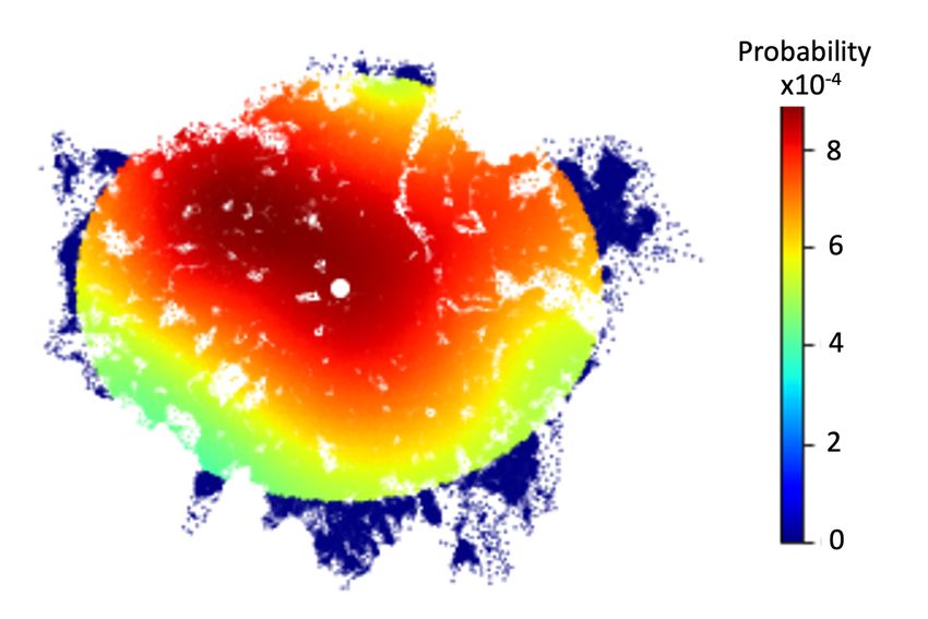
2
1.   Introduction

Understanding the interaction between business facilities and consumer preferences
is a prime factor of success for industries such as retail, healthcare and hospitality.
Therefore, accurate predictions of potential sales at business locations are becom-
ing crucial for planning and decision-making in the current ecosystem. Indeed,
the continuous growth in e-commerce (ONS, 2020) is threatening the existence of
traditional retail stores. We propose a Bayesian statistical methodology that, by
capturing the relationship between attractiveness of the facility, distance between a
business location and its customers, and demand in terms of buying power, allows
to make probabilistic forecasts about potential revenue at a business facility while
quantifying the uncertainty in these estimates.
    One of the earliest statistical models of customer behaviors when choosing shop-
ping facilities is a spatial interaction model, called Law of Retail Gravitation (Reilly
et al., 1929), which was inspired by the Newtonian gravity model and formulated a
customer’s choice between two facilities as a function of their attractiveness and dis-
tances. Huff (1963) subsequently extended this model to consider multiple facilities
while providing a probabilistic interpretation for the spatial interactions between
customers and facilities. In the following years, the Huff model (Huff, 1963) was
improved by replacing the single attractiveness term determined by floorspace with
a composite index of a set of attributes at the facility, including economic and struc-
tural factors (Nakanishi and Cooper, 1974; De Giovanni and Tadei, 2014). Most of
the literature estimates the parameters of spatial interaction models by resorting to
regression methods (Nakanishi and Cooper, 1974; Fotheringham and Webber, 1980;
Li and Liu, 2012; Bekti et al., 2018) or by maximising the entropy with respect
to some constraints (Fotheringham, 1983; Wilson, 2010). More recently, computa-
tionally intensive Markov Chain Monte Carlo (mcmc) schemes have been proposed
as an alternative inference method within the Bayesian framework for modelling
origin-destination flows but do not offer capabilities in estimating total revenue or
demand generated at the destination (Ellam et al., 2018; Congdon, 2010; LeSage
and Fischer, 2008).
    Inspired by the literature on gravity models, we develop a Bayesian spatial in-
teraction model, henceforth named bsim, which provides probabilistic predictions
about revenues generated at business facilities given their features and the potential
customers’ characteristics in a specified region in space. We model the probability
of a customer visiting each facility in a region through Gaussian densities in geo-
graphic space. Specifically, each density is centered on a facility with variance that
is further determined by its attractiveness which in turn modelled as a function of
internal and external characteristics (e.g. floorspace, distance to public transport
access points) and customer perspective (e.g. customer rating). The revenues for
each facility are then obtained by combining the probability of a customer visit with
a proxy of the individuals buying power, which we assume to be a function of their
socio-demographic characteristics. We adopt a Bayesian approach that enables us
to adequately account for the uncertainty associated with the customer interactions
with the facilities. Our framework not only gives accurate predictions but produces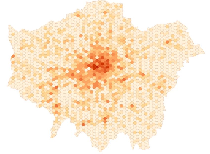
A Variational Bayesian Spatial Interaction Model    3
interpretable results that can support experts’ decision-making processes. More-
over, this approach allows us to infer quantities at the business facility or customer
level, such as revenue flow from customers to businesses. In bsim, the posterior
distributions of interest are intractable, and their approximation poses significant
computational challenges. We address this issue by resorting to variational inference
while also comparing with mcmc approximation. We demonstrate how our varia-
tional scheme is significantly faster compared to mcmc used in the literature while
providing comparable results in terms of parameter identification and uncertainty
quantification.

   In the literature, experiments on spatial interaction modelling are limited to
small synthetic datasets or real-world aggregated data since acquiring granular level
real-world data is usually expensive (Berman and Krass, 2002; Aboolian et al., 2007).
To address these constraints, we create a dataset that includes variables observed
at a granular level for public houses (pubs) and customers. This is performed by
combining large geospatial and non-geospatial data using open and commercial data
sources. Additionally, we gather customer reviews from Google’s customer rating
API, which covers a broader audience compared to the traditional survey meth-
ods found in the literature (Drezner, 2006). We demonstrate the benefits of the
proposed methodology on this real-world large scale dataset and show how bsim
outperforms competing approaches in terms of prediction performances. Further-
more, we illustrate how bsim provides interpretable results consistent with other
industry-related indicators observed for London.

   Our main contributions are: (a) we develop a Bayesian spatial interaction model
(bsim) that can be used to make probabilistic predictions of revenues or demand
generated at business facilities and formulates the relationship between distance and
attractiveness of facilities jointly, using a facility-specific probability distribution;
(b) we propose a scalable variational inference and demonstrate its benefits com-
pared to MCMC methods in a variety of experimental settings; (c) we construct an
unprecedented real-world large spatial dataset for pub activities at the most gran-
ular level along with customer characteristics at the postcode level, collated from
multiple sources; and (d) We show that our method provides the best predictive
performance compared to competing approaches while providing inference at the
level of customers and business facilities, delivering invaluable insights for planning
and decision making. To the best of our knowledge, we are the first to demonstrate
an application of a Bayesian spatial interactions model on a large scale real-world
dataset describing pub activities in the Greater London area with more than 1,500
business locations and 150,000 customer regions.

    This paper is organised as follows. In Section 2, we introduce bsim and the
related inference scheme. Then, we evaluate the model performance using syn-
thetic experiments in Section 3. In Section 4, we introduce a comprehensive spatial
database. Next, in Section 5, using the new dataset, we demonstrate the benefits of
our approach by inferring the model parameters for a real-world case study. Finally,
conclusions and future research directions are discussed in Section 6.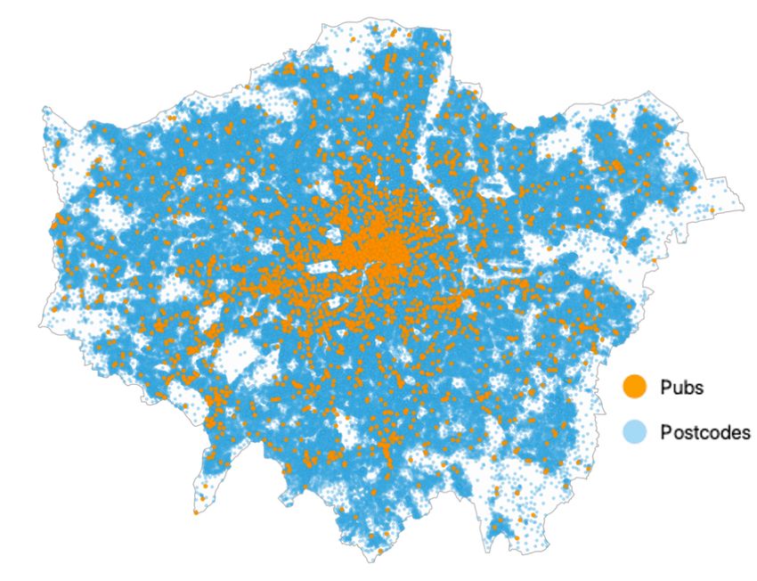
4
2. Methodology
We consider a regression problem for a given dataset D = {xs , ys }Ss=1 , where
xs ∈ RD represents the s-th store‡ features and ys ∈ R gives the revenue for
>
the s-th store in a bounded region τ . Each feature vector x> >
s = [ls , φs ] includes
the store location, which we denote by ls ∈ R2 , and additional store characteristics
denoted by φs ∈ RD−2 , e.g. floor size. For notational convenience we will denote
S × (D − 2) matrix of all stores characteristics by Φ. We assume the existence of
N customers within τ where vn is the n-th row of V ∈ RN ×P and represents the
features of the n-th customer. vn includes the customer location, which we denote
by mn ∈ R2 and its characteristics such as income level.
2.1. Model Formulation
The proposed Bayesian Spatial Interaction Model (bsim) is characterised by S Gaus-
sian distributions, one for each store, which are uncorrelated a priori. Each Gaussian
distribution, henceforth Zs ∼ N (µs , Σs ), is centered on a store’s location µs = ls
and has a diagonal covariance matrix Σs = σs2 I. The variance σs2 captures level of
“attraction” of a customer to a store. We propose two different alternative models
for variance. In the first model σs2 is written as a function of store specific coefficient
υs ∈ R that is:
σs2 = exp(υs ), (1)
In the second, we improve the specifications by denoting υs as a function of store
characteristics:
υs = λ> φs + εs , (2)
where λ ∈ RD−2 represents a shared coefficients across the stores and εs denotes
the unobservable store characteristics. Evaluating the probability density function
(pdf) of the variable Zs at mn , which we denote by Zs (mn ), allows us to capture
the likelihood for the n-th customer to visit the s-th store based on their distance
and on the store characteristics. For illustration purposes, consider three stores
where each has a Gaussian distribution centred on the store, as shown in Fig. 1.
Irrespective of the store’s attractiveness, customer behaviour is not affected after
a certain maximum distance to the store, known as “consideration set” in marketing.
Therefore, we truncate the Gaussian distributions in bsim and force their densities
to be zero beyond a given distance dT from the store location. The truncated
Gaussian pdf is given by:
exp −d2ns /2σs2
, 0 ≤ dns ≤ dT ,
Zs (mn ) = 2πσs2 1 − exp (−d2T /2σs2 ) (3)
0, otherwise,
where dns denotes the Euclidean distance between the store and customer dns =
||mn −ls ||2 ; see Appendix A for details. Fig. 2 demonstrates the truncated Gaussian
densities corresponding to the distributions shown in Fig. 1.
‡We present the rest of the model in relation to the specific instantiation where a business
location is a store, but this can be extended to other business facilities.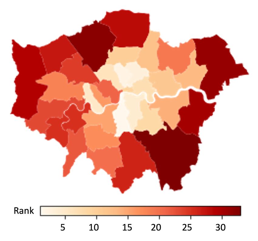
A Variational Bayesian Spatial Interaction Model      5

                          (a)                                  (b)

Fig. 1. Illustration of the PDF of the Gaussian distribution centered on three sample Stores
: (a) 3D visualisation; (b) 2D visualisation. The white dots indicate the store location and
the numbers are used to identify the respective stores on 3D and 2D visualisations.

                          (a)                                  (b)

Fig. 2. Illustration of the Truncated Gaussian centered on three sample Stores: (a) 3D
visualisation; (b) 2D visualisation. The white dots indicate the store location. There is a
hard border around the distributions beyond which the PDF is equal to zero.

   Given the truncated Gaussian distributions, we define the probability pns of a
customer visiting the s-th store as:

                                          Zs (mn )
                                  pns = PS            .                                 (4)
                                         j=1 Zj (mn )

   Note that we normalize the pdf calculated for the customer with respect to the
store by the total pdf respect to all the stores within the consideration set to arrive
6
at a value which falls in the interval of [0, 1]. Thus we assume that every customer
chooses at least one store in their consideration set, but this can be relaxed by
adding pseudo stores to account for unsatisfied demand or unobserved data. The
value of pns capture the level of competition in the region τ for a specific type of
store. For instance, pns will be lower in competitive markets or areas while it will
take higher values in non-competitive settings. This is illustrated in Fig. 3 with
respect to the non-truncated and truncated Gaussian distributions.

                                              (a)

                                              (b)

Fig. 3. Illustration of the probability of customers visiting a store pns : (a) with none trun-
cated Gaussian distribution; (b) with truncated Gaussian distribution. This is an indication
of the competition in the area. The white dots indicate the store location, and the numbers
are used to identify the respective stores on (a) and (b) plots.

   The consumption function in economics determines the relationship between
consumer spending and the various factors (Modigliani and Brumberg, 1954). To
model the amount budgeted by each customer for spending we propose a linear
function f (·) which takes input vn [−mn ] representing the P − 2 customer features
obtained by discarding the location coordinates:

                            rn = f (vn [−mn ]) = β T vn [−mn ],                            (5)

where β ∈ RP −2 . This leads to the conventional Spatial interaction system (Huff,
1963; Wilson, 1971; Ellam et al., 2018). Thus expenditure flow from customer n to
store s:

                                      rns = rn × pns ,                                     (6)

where the amount each customer budgeted to spend rn is weighed by the probability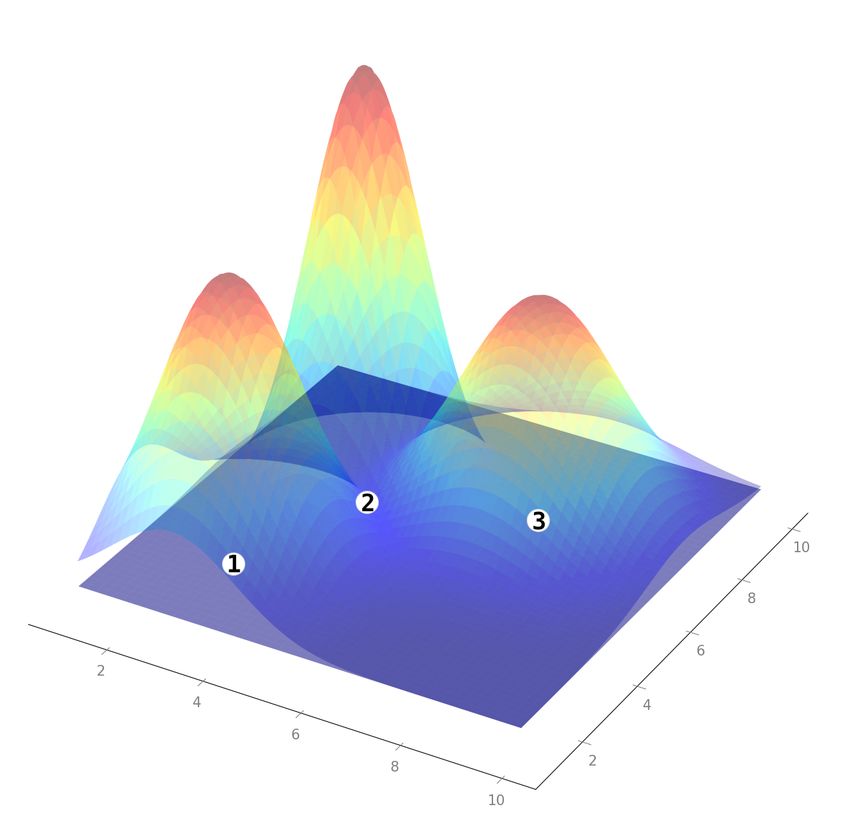
A Variational Bayesian Spatial Interaction Model      7
to visit the s-th store. The total revenue for the s-th store is:
                         N                N
                         X                X                   Zs (mn )
                  rs =         rn pns =       β T vn [−mn ] PS            .                (7)
                         n=1              n=1                j=1 Zj (mn )

   Henceforth we derive the model for the case where the store variance is a func-
tion of its features (Eq. (2)), since the limiting case where the store variance is store
specific coefficient (Eq. (1)) is a trivial extension by setting λ to zero.

Likelihood function:           The likelihood of the observed stores’ revenue Y = {y1 , . . . , yS }
is defined as:
                                                  S
                                                  Y
                          p(Y|β, λ, ε, σ 2 ) =          N (ys ; rs , σ 2 ),                (8)
                                                  s=1

where the model assumes constant-variance (σ 2 ) for the Gaussian noise.

Prior Distributions: We assign prior distributions to all model parameters.
First, we define a hierarchical prior distribution for β, which we assume to be a
Gaussian with mean µβ and covariance α−1 I:
                                  p(β|α) = N (β; µβ , α−1 I),
Following the standard practices, we introduce a Gamma prior distribution with
shape ω1 > 0 and scale ω2 > 0 for the hyper-parameter α:
                                   p(α) = Gam(α; ω1 , ω2 )
Similarly, we assign a Gamma prior distribution with shape ρ1 and scale ρ2 for the
likelihood precision parameter γ = σ −2 :
                                   p(γ) = Gam(γ; ρ1 , ρ2 ),
Finally, the following Gaussian prior distributions are selected for λ and ε with
mean µ and covariance %I,
                                    p(λ) = N (λ; µλ , %λ I)
                                    p(ε) = N (ε; µε , %ε I).

Posterior Distribution: The full vector of model parameters is denoted by
Θ = {β, λ, ε, γ}. Posterior probability given by:
                                                p(D|Θ)p(Θ)
                                p(Θ|D) = R                                                 (9)
                                               p(D|Θ)p(Θ)dΘ
where the marginal density takes the form:
            Z     Z
     p(D) = · · · p(D|β, λ, γ)p(β|α)p(α)p(λ)p(ε)p(γ) dβ dα dλ dε dγ.                      (10)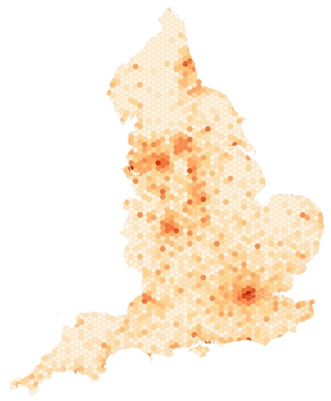
8
                                                                                µβ
    %λ                                                                           .        ω2
     .                                                                                     .

    µε                                                                                    ω1
     .         εs          σs2 I      mn          vn [−mn ]         β           α          .

                                                                    P-2
    %λ                                                                                   ρ2
     .                                                     N                              .

    µλ                                                                                   ρ1
     .          λ          φs          ls             ys                       γ          .

                           D-2                                          S

Fig. 4. Plate diagram for the graphical representation for the BSIM. Specifically, this express
the spatial interaction between S number of stores with each store revenue ys , located at
ls with store features φs and N number of customers located at mn with P-2 characteristics
vn [−mn ]. We use Gaussian distributions as priors for β, λ, ε and Gamma distributions for
γ, α. The diagram represents random variables with circles ( ), known values with grey
filled circles ( ) while black filled circles ( ) indicate fixed parameters of prior and hyper-
prior distributions, edges denote possible dependence, and plates denote replication.

2.2. Inference
Our goal is to estimate the posterior distribution over all parameters given the data
i.e. p(Θ|D). Since marginal density is analytically intractable (Eq. 10), we resort
to approximate inference by employing two commonly used methods: Variational
Inference (VI) (Jordan et al., 1999) and Markov Chain Monte Carlo (mcmc) (Hast-
ings, 1970).
2.2.1. Variational Inference
vi is a powerful method to approximate intractable integrals where in contrast to
mcmc, it tends to be much faster because it rests on optimisation instead of sampling
(Blei et al., 2017). VI first posits a family of densities and then finds the member of
that family, which is closest to the posterior by minimizing the Kullback-Leiber (kl)
divergence. Because the kl divergence cannot be directly calculated, alternatively,
we maximise evidence lower bound, Lelbo that is equivalent to minimizing the kl
divergence.

Variational Distributions: We use the mean-field approximation and assumed
a fully factorized variational distribution (Bishop, 2006):
                         q(β, α, γ, λ, ε) = q(β)q(α)q(γ)q(λ)q(ε),                         (11)
with
                                    q(β) = N (β; µˆβ , Ω)                                 (12)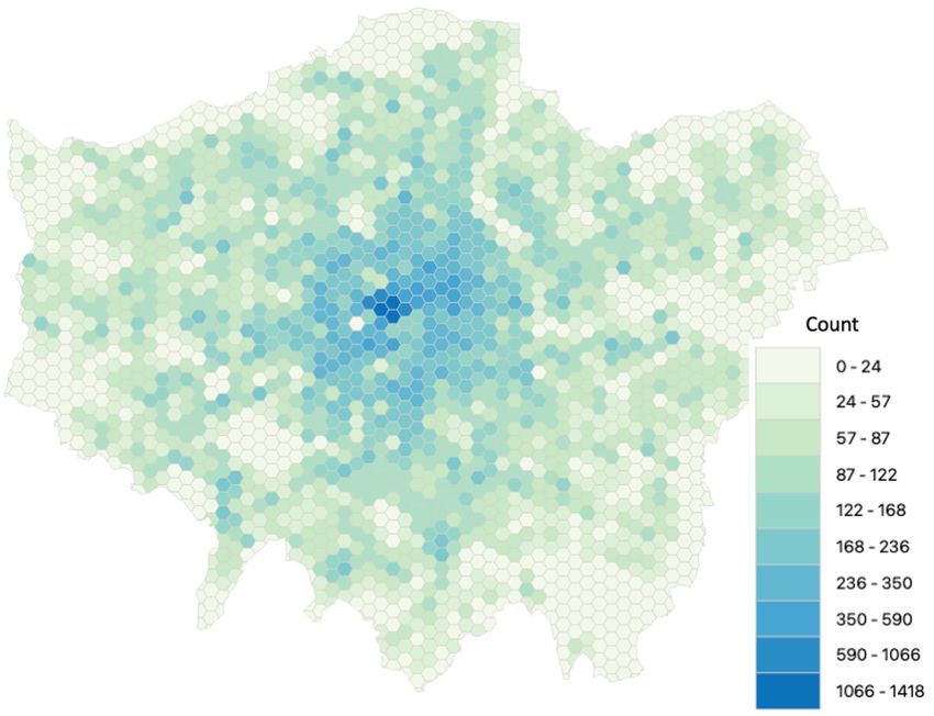
A Variational Bayesian Spatial Interaction Model 9
q(α) = Gam(α; ωˆ1 , ωˆ2 ), (13)
q(γ) = Gam(γ; ρ̂1 , ρ̂2 ), (14)
q(λ) = N (λ; µˆλ , Kλ ), (15)
q(ε) = N (ε; µˆε , Kε ), (16)
where ν = {µˆβ , Ω, ωˆ1 , ωˆ2 , ρ̂1 , ρ̂2 , µˆλ , Kλ , µˆε , Kε } are the variational parameters
which are optimized within the algorithm. Eqs. (12)–(16) define our approximate
posterior. With this, we give details of the variational objective function, i.e. elbo,
which we aim to maximize with respect to ν.
Evidence Lower Bound: Following the standard variational inference, elbo
can be written as a combination of expected log likelihood (Lell ) and kl-divergence
term (Lkl ):
Lelbo (ν) = Lell (ν) − Lkl (ν). (17)
the expected log likelihood term can be written as
Lell = Eβ,γ,λ,ε [ln p(Y |β, γ, λ, ε)]
S S
=− ln 2π + (ψ(ρ̂1 ) − ln ρ̂2 )− (18)
2 2
S N
!2
1 ρ̂1 γ X X Zs (mn )
Eβ,γ,λ,ε ys − β > vn [−mn ] PS
2 ρ̂2 2 j=1 Z j (mn )
s=1 n=1
the kl-Divergence Term is expanded and simplified as:
Lkl = E[ln p(Θ)] − E[ln q(Θ)]
= Eβ,α [ln(p(β|α)] + Eα [ln p(α)] + Eλ [ln p(λ)] + Eε [ln p(ε)] + Eγ [ln p(γ)]− (19)
Eβ [ln q(β)] − Eα [ln q(α)] − Eλ [ln q(λ)] − Eε [ln q(ε)] − Eγ [ln q(γ)],
where each term is given in the Appendix A. Lelbo (ν) is not computable in analyti-
cally closed forms and remains intractable. Hence we resort to Black Box variational
inference method where the gradient is computed from the Monte Carlo samples
from the variational distributions (Ranganath et al., 2014). We implement the al-
gorithm using Tensorflow 2 (Abadi et al., 2016) in Python 3.
2.2.2. Markov Chain Monte Carlo
In order to compare our estimations we describe the mcmc which has been the
dominant paradigm for approximate inference for decades. First, we construct a
Markov chain on Θ whose stationary distribution is the posterior p(Θ|D). Then we
collect samples from the stationary distribution by sampling from the Markov chain.
Finally, we use the collected samples to approximate the posterior with an empirical
estimate. mcmc methods ensure producing exact samples from the target density
but tend to be computationally intensive (Robert and Casella, 2013). When the
datasets are large, mcmc becomes slower and computationally expensive to form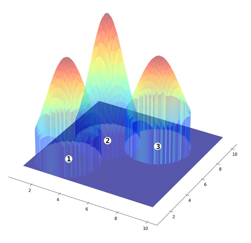
10
inferences. We use open-source software, Stan which is a C++ library for Bayesian
modeling, with the R interface to compile results (Stan Development Team, 2020).
We adopt the No-U-Turn sampling method, an extension to Hamiltonian Monte
Carlo algorithm for the experiments (Hoffman et al., 2014).

2.3. Edge Correction
Stores on the edge of the study area τ cannot be evaluated without a certain bias
because the model cannot capture the contribution from customers living outside τ .
To overcome this, we adjust the revenues of the stores {ys }Ss=1 , and this is carried
out before fitting the model. Following a similar approach to the model, we assume
a Gaussian centered on the store and calculate the area under the curve (auc) A,
which intersects with the study area. We set the variance η 2 of the Gaussian to be
dT /4 to cover approximately an area of 0.99 within the buffer radius of dT around
the store center ls . Calculating the auc for an arbitrary polygon as shown in Fig. 5,
is computationally challenging. Henceforth we use the Monte Carlo method, where
the samples are drawn from N (ls , η 2 I) and reject them if outside the τ to calculate
the fraction of kept samples.

Fig. 5. The red marker denotes a store at the edge of London. There may be customers
who contributes to its revenue but not in the study area. Intersection of the radius and
London map results in an arbitrary polygon shape.

     We formulate the adjusted revenue yes as the actual revenue weighted by the auc:
                                     yes = ys × A.                                 (20)
We apply this to real-world data for edge correction before fitting the bsim.

3.    Simulation study
We design a simulation study to examine the inferences obtained from vi and mcmc
methods under different synthetic settings characterised by an increasing number of
stores and customers. We also compare the computational performance of the two
methods by observing the run time of each fitted model. First, we simulate the data
from a spatial process that closely matches the modeling framework introduced in
Section 2, Eq. (2) with εs = 0. The process is defined as:
                               ys |β, λ, σ 2 ∼ N (rs , σ 2 ),                      (21)
A Variational Bayesian Spatial Interaction Model 11
Table 1. The first row indicates the True values of the parameters used to create the syn-
thetic data, and the following rows display the first (Mean) and second moments (Standard
deviation) along with its 95% quantile-based Credible Intervals (CI) for the posterior distri-
butions for VI and MCMC methods.
β1 β2 λ1 λ2 γ
True −0.2 0.4 0.1 0.5 4
Mean −0.196 0.398 0.164 0.383 1.821
vi Std 0.014 0.018 0.235 0.116 0.727
CI (−0.224, −0.169) (0.362,0.434) (−0.296, 0.625) (0.156, 0.609) (0.687, 3.499)
Mean −0.198 0.400 0.185 0.387 1.908
mcmc Std 0.017 0.021 0.547 0.393 0.904
CI (−0.235, −0.166) (0.358 , 0.447) (−0.839, 1.387 ) (−0.313, 1.269) (0.562, 4.054)
where the locations of stores and customers are simulated within a square. Two
customer features are generated, one with a strong spatial correlation and the other
with a moderate spatial correlation to closely reflect the real-world customer features
as shown in Fig. 6. The store locations are randomly sampled within the same
spatial boundaries used to sample the customers. Store features are sampled from
a Gamma distribution (Φ ∼ Gam(1, 1)) to represent features such as floorspace.
(a) (b)
Fig. 6. Simulated Customer features for N = 1000 under two different spatial correlation
structures to closely simulate the real-world scenarios: (a) Strong Spatial Correlation; (b)
Moderate Spatial Correlation.
3.1. Parameter Estimation
For both vi and mcmc methods, all priors are chosen to be weakly informative to
allow the data to drive the inference as illustrated in Table 2. We fit our mcmc
model using one chain with 5000 iterations by removing the first 2500 for warm-
up, and every post-warm-up iteration is used for posterior samples. The posterior
distributions along with the prior distributions are visualised in Table 2 and pa-
rameter estimates are presented in Table 1. The results indicate that both methods
approximate the posterior mean effectively and variational approximations of the
posterior variance are lower than mcmc method.12
Table 2. Column one demonstrates the weakly informative prior distributions, and the
following columns illustrate marginal posteriors of the interested parameters inferred
by VI and MCMC. Synthetic experiment consists of 10 stores and 1000 customers
(S = 10, N = 1000).
Prior vi vs. mcmc
−1
p(β|α) ∼ N (0, α I) β1 β2
p(α) ∼ Γ(1, 1)
p(λ) ∼ N (0, α−1 I) λ1 λ2
p(γ) ∼ Γ(1, 1) γA Variational Bayesian Spatial Interaction Model 13
The simulation process explained above is experimented under two different syn-
thetic settings:
(a) sim1 : 10 stores with 1000 individuals (S = 10, N = 1000)
(b) sim2 : 50 stores with 2000 individuals (S = 50, N = 2000)
We simulate random store locations to create 50 datasets and compare the per-
formance across datasets using the posterior means of β, λ, γ and the 95% quantile-
based credible intervals for each parameter from each fitted model. Three standard
measures are used to compare the performance between mcmc and vi methods:
(a) the bias, which measures the differences between the posterior mean from
the model fit to dataseti (β̂i ) and the true value of the parameter β, Bias =
1 P50
50 i=1 (β̂i − β);
(b) the mean-squared error (mse), which takes the squared of the difference be-
1 P50 2
tween posterior mean and true value, mse = 50 i=1 (β̂i − β) ;
(c) the coverage of the 95% quantile-based credible interval obtained from fitting
1 P50
the model to dataseti , coverage = 50 i=1 I (β ∈ credible intervali ), where I(·)
is the indicator function equal to 1 if the statement is true and 0 otherwise.
Table 3 and Table 4 show the results of the fitted models for the two synthetic
settings, averaged across the 50 datasets. Both vi and mcmc algorithms exhibit
comparable performance in terms of bias, mse, and coverage across both simulation
studies. For sim1 , we observe lower coverage for γ with the vi scheme. However
the coverage for γ is improved to one in the sim2 . Both λ and γ parameters result
in a higher estimated mse under both the simulation setting for vi and mcmc
methods. This is an indication of the lack of identifiability in the parameters due
to the flexibility in the model. The precision γ of the error term σ 2 tends to be
underestimated on average. Both models are fitted on a Intel Xeon CPU (3.5GHz
and 32 GB of RAM). The run time of the vi algorithm is about five times faster than
the mcmc algorithm in the simulation study. This is vital for our real-world data
application, where the number of spatial locations is much larger than the synthetic
settings. Overall the vi algorithm exhibited a reduced run time while providing good
estimations and inference of the parameters of interest in this simulation study.
3.2. Model Comparison
Finally under the simulation study, we conduct a comparison of our model with the
Huff modified model (Li and Liu, 2012). Two standard metrics are used to evaluate
the performance:
(a) the Normalised Root-Mean-Squared Error (nrmse), which measures the dif-
ferences between
√the values predicted by a model (Ŷ) and the values observed
E[Y−Ŷ]2
(Y), nrmse = E[Y] ;14
Table 3. VI and MCMC simulation study performance for S = 10, N = 1000.
Metric Method β1 β2 λ1 λ2 γ
vi −0.002 0.004 0.258 0.110 −1.828
Bias
mcmc −0.002 0.004 0.265 0.116 −1.772
vi 0.000 0.000 0.130 0.051 3.467
mse
mcmc 0.000 0.42 0.130 0.049 3.276
vi 0.94 0.96 1. 1. 0.44
Coverage
mcmc 0.96 0.98 1. 1. 0.94
vi mcmc
Run time (s)
207 1064
Table 4. VI and MCMC simulation study performance for S = 50, N = 2000.
Metric Method β1 β2 λ1 λ2 γ
vi 0.000 0.002 −0.338 0.352 −0.754
Bias
mcmc 0.002 -0.001 −0.092 0.341 −0.734
vi 0.000 0.000 0.185 0.179 0.598
mse
mcmc 0.000 0.000 0.008 0.186 0.571
vi 1. 0.94 0.84 0.94 1.
Coverage
mcmc 1. 1. 1. 0.857 1.
vi mcmc
Run time (s)
1079 5280
(b) the R-squared, which is the ratio of the variance of the residuals (SSres ) and
he variance of the observed Y (SStot ), R2 = 1 − SS
SStot .
res
Table 5 displays the results for bsim and Huff modified model. bsim exhibits
better performance across both the settings compared to the modified Huff model.
We observe an increase in nrmse for both models as the number of stores and
customers increases. However, the R2 remains unaffected at significantly high levels
showing more robust performance for bsim under both simulation settings compared
to the modified Huff model.
Table 5. Performance of the simulation studies for BSIM and Huff
modified model. sim1 : S = 10, N = 1000 and sim2 : S =
50, N = 2000 .
sim1 sim2
Model 0.98 0.94
R2
Modified Huff Model 0.77 0.30
Model 0.07 0.15
NRMSE
Modified Huff Model 0.24 0.64A Variational Bayesian Spatial Interaction Model 15
4. Large-scale geospatial dataset of pub activities in London
We initially develop a large-scale, geospatial dataset for England non-domestic prop-
erties using data from multiple sources. However, for the interest of this study, we
limit to one non-domestic property category, public houses (pubs), which are lo-
cated in Greater London. To the best of our knowledge, this is the first study
exploring these datasets together to benefit retail businesses. A detailed descrip-
tion of each dataset is given in Appendix B. All the spatial data processing is done
using PostGIS on a PostgreSQL database.
4.1. Store level data
We compile a dataset with stores’ geospatial location, rateable values, and store-
specific features. We do this by Joining the VOA (Valuation Office Agency, 2019)
and Addressbase from Ordnance Survey (2019) data using the cross-reference which
renders all of the non-domestic properties geo-coordinates and their rateable values.
The calculation of the rateable values of pubs is different from other categories. In
contrast, the rateable value of pubs is based on the annual level of trade (exclud-
ing VAT) that a pub is expected to gain if operated in a reasonably efficient way
(Valuation Office Agency, 2016). Hence the rateable value is a good proxy of the
pub revenues, and we use data related to pubs for the real-world experiment in this
study. There are 40,000 pubs recorded in VOA for England and Wales. The spatial
distribution of pubs across England is shown in Fig. 7.
(a) (b)
Fig. 7. Spatial distribution of pubs: (a) across England; (b) zoomed into Greater London.
The region is split into equal size grids of hexagons (size of each side : (a) 5km; (b) 0.5km)
and number of pubs within each hexagon is displayed with a colour gradient.16
The store features are an essential factor in assessing the attractiveness of the
stores. The internal store characteristics of the building, such as the floor size,
height are extracted from the OS Mastermaps from Ordnance Survey (2020). This
is accomplished by first spatially joining the polygon of the land (HM Land Registry,
2020) with locations of stores and next spatially join the polygon of the footprint
from Mastermaps. Additionally, external characteristics such as the closest distance
to public transport access points (Department for Transport, 2014), tourist attrac-
tions (Historic England, 2014) are calculated using the Euclidean distance between
spatial locations. We have strengthened the store attractiveness measures by using
the customer reviews on Google (Google, 2020). People can write reviews and rate
the places voluntarily on Google maps. The ratings are then aggregated and shown
to the public. Using the Google Places API, this data can be accessed at a cost.
Flow diagram of the process used to extract the store features are demonstrated in
Fig. 8.
Ordnance Survey Ordnance Survey OS Addressbase
Addressbase MasterMaps
Spatial Join
Land Registry
National Polygons
OS Mastermaps
Cross reference
National Polygon
Valuation Office OS Addressbase
Agency Google
Business Rates
Google
Place API
National Polygon
Fig. 8. Diagram illustrates the steps to extract the store features. Each dataset is named as
per the data source along with its number of records (obs) or size. Initially OS addressbase
is joined with VOA dataset and then spatially joined with National Polygons data to find the
Title polygon of each land. This is next joined with Mastermaps and linked with Google
data to obtain the store footprints and google customer ratings respectively.
4.1.1. Customer level data
The most granular level of customer data can be identified as the residential loca-
tions. OS Addressbase dataset provides both residential and commercial addresses
(over 40 million) along with geo-locations. However, since there is no data for cus-
tomer features at the residential level, in this study, we use postcodes which is the
next most granular level. Henceforth, we assume that the customers’ behaviour who
are residing in the same postcode are homogeneous. In Greater London on average
there are 17 households per postcode. The postcode centroids for Greater LondonA Variational Bayesian Spatial Interaction Model 17
are displayed in Fig. 9. The population and proportion of gender at the postcode
level are used to reflect the demographics in the area. Additionally, we employ the
deprivation data to understand the customer characteristics in the area (Ministry
of Housing, Communities & Local Government, 2019). There are seven domains of
deprivation categories: (1) Income Deprivation, (2) Employment Deprivation, (3)
Education, Skills and Training Deprivation, (4) Health Deprivation and Disability,
(5) Crime, (6) Barriers to Housing and Services and (7) Living Environment De-
privation. Deprivation level data is provided at the LSOA level. We assign that to
the postcodes by point to polygon spatial join.
5. Case study: estimating revenues of pubs in London
In this section, we illustrate our proposed methodology using the pubs’ dataset
developed for Greater London in section 4. After compiling data from different
sources, the final complete dataset consists of S = 1804 pubs. The derived approxi-
mated revenue after adjusting for edge correction (Eq. (20)) is used as the response
variable ys in the model with natural log transformation. For each pub, we derived
pub-specific features: floorspace, height, number of floors, the total area of land;
distance to the closest metro, train station, bus stop, park, popular attractions,
sports facility; customer rating on Google, number of users rated and an indicator
to show if the pub is in a major town.
We determine the customer locations at the postcode level, which is the most
granular level of census estimates are released. There are N = 174360 postcodes for
Greater London. We represent the characteristics of the postcodes by the population
at each postcode and its proportion of male, and deprivation scores. All features
have been normalized before training the model. The model may be improved
with more granular customer-specific characteristics; underlying arguments would
remain the same. Centroids of the postcodes and retail locations of the pubs are
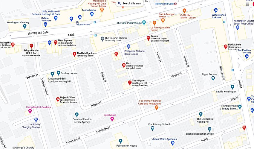
presented in Fig. 9(a), on a map of London.
(a) (b)
Fig. 9. (a) Visualization of the locations of pubs in orange markers (S = 1804) and postcode
centroids in blue markers (N = 174360) over the map of London; (b) Greater London is split
into equal size grids of hexagons (size of each side is 0.5km) and number of postcodes
within each hexagon is displayed with a colour gradient.18
(a) (b) (c)
Fig. 10. Demonstration of different radius used for truncated Gaussian with an example
concerning a pub located in the center of London. Three radii were used in the study: (a)
15km; (b) 20km; (c) 25km.
Table 6. R2 , σ 2 and NRMSE for the fitted BSIM with rev-
enues of pubs in Greater London under three different
radii of the truncated Gaussian.
Truncated radius (km)
15 20 25
R2 0.19 0.72 0.57
σ2 0.67 0.45 0.52
nrmse 0.08 0.05 0.06
Customer behavior is not affected after a certain distance from the business
facility, despite the pubs’ attractiveness. We explore the model under three dif-
ferent radius, dT = 15km, 20km and 25km as presented in Fig. 10. We calculate
the distance between origin and pub using Euclidean distance, although a better
representation would use a transport network.
We first perform a preliminary study of our model with a store-specific coefficient
which denotes the store-specific variance σs2 = exp(υs ), representing the attractive-
ness of the store as given by Eq. (1). We experiment with the model for three
different radii of the truncated Gaussian and model performance summarised in
Table 6. Results indicate that R2 increased to 0.72 as the radius increased from
15km to 20km but reduced to 0.57 as the radius increased to 25km. Hence the best
experimental results yielded for truncated Gaussian with a radius of 20km.
Next, we perform a detailed study on the model with improved specifications
where store features represent the attractiveness of the store (Eq. (2)). In this
study, the radius of the truncated Gaussian is set to 20km, as it demonstrated the
best results for the previous experiment. The model with these settings resulted in
a high R2 of 0.88 and a low nrmse of 0.03. The plots (Fig. 11) of the observed
revenue and predicted revenues suggest that the model provides a good fit to the
data. The residuals are relatively high out of central London, closer to a major
ringway as shown in Fig. 11 c. Additionally, the predicted revenue of a few pubs at
the edge of the study area is underestimated, reflecting the edge effects.
Using the parameter estimates (λ, ε) from the best-fitted model, we have demon-A Variational Bayesian Spatial Interaction Model 19
(a) (b)
14
13
12
11
E(ys|x, D)
10
9
8
7
7 8 9 10 11 12 13 14
ln(ys)
(c) (d)
Fig. 11. Visualisation of the Pub’s revenue and predictions over greater London map with
truncated Gaussian radius of 20 km: (a) Revenue at each pub; (b) Predicted revenue at
each pub; (c) Residuals marked in points and lines are the major roads; (d) Actual against
predicted revenue. The experiment resulted in R2 = 0.88 and NRMSE = 0.03.
strated the attractiveness (σs2 ) of pubs around London in Fig. 12(a). It can be ob-
served that the most attractive pubs are within or around the major towns. Further
exploring the coefficients of pub features, we found that Google’s customer rating
score and the number of people rated had the highest positive contribution towards
the attraction term (Appendix C). This implies that customer rating is a critical
indicator in describing the customer attractiveness to the pubs. The remaining term
used to express the attractiveness, unobserved pub features (εs ), where the abso-
lute coefficient is mapped in Fig. 12(b). There is a similar pattern to the residual
plot, but overall spatial distribution appears to be random. A deep investigation is
required to understand what could explain the unobserved pub features.
For demonstration purposes, we randomly select a pub in central London to
explore the insights from the fitted model. The probability of people within the20
(a) (b)
Fig. 12. Exploring the pubs attractiveness for the fitted model: (a) Variance (σs2 ) of the
Gaussian placed on each pub. Blue colour polygons denote the major towns; (b) Absolute
coefficients of the unobserved pub characteristics (εs ).
postcode selecting the particular pub (pns ) is calculated using the model parameter
estimates with Eq. (4). These probabilities are mapped into a heatmap as shown
in Fig. 13. There appear to be two hotspots on the map, one closer to the pub, and
another one towards North-West London. It is natural to see higher probabilities
closer to the pub, but the other hotspot is possible because the pubs’ density in
the area is comparatively low, as shown in Fig. 9(a). Hence people in the area also
prefer traveling to pubs in central London. The distribution of probabilities tends
to be having an oval shape, possibly because the distance between the customers
and pubs is calculated as Euclidean distance. A better representation could occur
in using a transport network.
Fig. 13. Visualisation of the probability (pns ) of people in each postcode selecting the
particular pub shown in a white dot in the centre of London.A Variational Bayesian Spatial Interaction Model 21
Using the parameter estimates (β) from the best-fitted model, we can estimate
the amount spent by customers living in each postcode (rn ). Coefficients of the
deprivation features indicate that areas with higher income, high employment, less
risk of crimes, better quality of life, and environment tend to positively influence
the customers’ spending levels at pubs. The amount spent at each Borough can be
derived by calculating the total of the estimated spending amount at each postcode
within the Borough. This we compare against the alcohol-related mortality in the
London Boroughs published by Public Health England (2021). The rank of Bor-
oughs respective to the spending and mortality levels published for 2017 is mapped
in Fig. 14. The rank correlation between mortality count and estimated spending
shows a moderate positive relationship of 0.4. Our intuition is that higher alcohol-
related mortalities are to be expected in the areas of high alcohol consumption.
(a) (b)
Fig. 14. Visualisation of ranking on estimated revenue and mortality in the London Bor-
oughs : (a) Rank of estimated amount spent at the pubs by people living in each Borough;
(b) Rank of Mortality count.
Finally, we perform a comparison with a spatial interaction model from the
literature for completeness of the study. We fitted the Modified Huff model (Li and
Liu, 2012) for the same dataset, which displayed very low performance with R2 of
only 0.03 and nrmse of 0.84. Our model outperforms the benchmark model with a
notable improvement and provides valuable inferences for decision-makers.
6. Discussion
We have developed a Bayesian spatial interaction model to simulate customers’
behavior with business facilities using their respective characteristics. bsim consid-
erably improves existing classical Huff type models as it formally addresses uncer-
tainties arising in the modelling process, via a Bayesian framework while providing
inferences at the level of business and customer locations. The key advantage of the
proposed model is scalable and can make inference on large-scale datasets through22
deterministic variational inference, in contrast to the existing models. The synthetic
experiments show how vi performs five times faster than mcmc while providing com-
parable performances in terms of parameter identification and without significant
under estimation of the posterior covaraince.
For the first time, we are able to demonstrate and estimate spatial interactions
in large real-world urban extend such as Greater London with more than 1500
pubs and 150000 customer regions. For this purpose, we develop a large dataset
at the most granular level by utilising data from multiple sources. We presented
our methodology in the context of Pubs, but this can be applied in other retail
businesses or even expand into sectors such as healthcare and energy. Furthermore,
we demonstrate that bsim can infer different components of the spatial interactions,
thereby making valuable conclusions for a businesses’ ability to make decisions.
Finally, we have shown how bsim outperforms competing approaches in terms of
prediction performances while providing consistent results with related indicators
observed for the London region.
The proposed methodology can be extended and improved upon across multiple
dimensions. First, one could consider adopting a travel network to estimate the
distance instead of the Euclidean metric used in this study (Lafferty et al., 2005;
Grigoryan, 2009; Crosby et al., 2018). This could provide a more realistic con-
figuration of the geographical setting and lead to better inferences. Furthermore,
extending the proposed framework to a spatio-temporal setting to capture the time
evolution of parameters to understand the behavioural changes of customers and
changes in urban systems will also be of significant interest. Lastly, our work opens
up the potential to utilise the bsim to select the optimal business location.
7. Acknowledgements
We would like to thank the UK Engineering and Physical Sciences Research Council
(EPSRC grant no. EP/L016710/1 and EP/R512229/1). Furthermore, this work
was supported by the Alan Turing Institute under EPSRC grant EP/N510129/1,
UKRI Turing AI fellowship EP/V02678X/1, and the Lloyds Register Foundation.
We are also grateful to Nimbus property system limited for their support and giving
access to a comprehensive property database, and for the valuable insights shared
by its Director, Paul Davis.
References
Abadi, M., Agarwal, A., Barham, P., Brevdo, E., Chen, Z., Citro, C., Corrado,
G. S., Davis, A., Dean, J., Devin, M. et al. (2016) Tensorflow: Large-scale machine
learning on heterogeneous distributed systems. arXiv preprint arXiv:1603.04467.
Aboolian, R., Berman, O. and Krass, D. (2007) Competitive facility location model
with concave demand. European Journal of Operational Research, 181, 598–619.
Bekti, R., Pratiwi, N. and Jatipaningrum, M. (2018) Multiplicative competition
interaction model to obtained retail consumer choice based on spatial analysis. InA Variational Bayesian Spatial Interaction Model 23 IOP Conference Series: Earth and Environmental Science, vol. 187, 012041. IOP Publishing. Berman, O. and Krass, D. (2002) Locating multiple competitive facilities: spatial interaction models with variable expenditures. Annals of Operations Research, 111, 197–225. Bishop, C. (2006) Pattern Recognition and Machine Learning. Information Science and Statistics. Springer. Blei, D. M., Kucukelbir, A. and McAuliffe, J. D. (2017) Variational inference: A review for statisticians. Journal of the American statistical Association, 112, 859–877. Congdon, P. (2010) Random-effects models for migration attractivity and retentiv- ity: a bayesian methodology. Journal of the Royal Statistical Society: Series A (Statistics in Society), 173, 755–774. Crosby, H., Damoulas, T., Caton, A., Davis, P., Porto de Albuquerque, J. and Jarvis, S. A. (2018) Road distance and travel time for an improved house price kriging predictor. Geo-Spatial Information Science, 21, 185–194. De Giovanni, L. and Tadei, R. (2014) Modeling the retail system competition. Procedia-Social and Behavioral Sciences, 108, 285–295. Department for Transport (2014) National Public Transport Access Nodes (NaPTAN). URL: https : / / data . gov . uk / dataset / ff93ffc1 - 6656 - 47d8 - 9155 - 85ea0b8f2251/national-public-transport-access-nodes-naptan. Drezner, T. (2006) Derived attractiveness of shopping malls. IMA Journal of Man- agement Mathematics, 17, 349–358. Ellam, L., Girolami, M., Pavliotis, G. A. and Wilson, A. (2018) Stochastic modelling of urban structure. Proceedings of the Royal Society A: Mathematical, Physical and Engineering Sciences, 474, 20170700. Fotheringham, A. S. (1983) A new set of spatial-interaction models: the theory of competing destinations. Environment and Planning A: Economy and Space, 15, 15–36. Fotheringham, A. S. and Webber, M. J. (1980) Spatial structure and the parameters of spatial interaction models. Geographical Analysis, 12, 33–46. Google (2020) Place Search. URL: https://developers.google.com/places/web- service/search. Grigoryan, A. (2009) Heat kernel and analysis on manifolds, vol. 47. American Mathematical Soc. Hastings, W. K. (1970) Monte carlo sampling methods using markov chains and their applications.
24
Historic England (2014) Listing. URL: https://historicengland.org.uk/listing/the-
  list/.
HM Land Registry (2020) National polygon service. URL: https://www.gov.uk/
 guidance/national-polygon-service.
Hoffman, M. D., Gelman, A. et al. (2014) The no-u-turn sampler: adaptively setting
 path lengths in hamiltonian monte carlo. J. Mach. Learn. Res., 15, 1593–1623.
Huff, D. L. (1963) A Probabilistic Analysis of Shopping Center Trade Areas. Land
 Economics, 39, 81.
Jordan, M. I., Ghahramani, Z., Jaakkola, T. S. and Saul, L. K. (1999) An introduc-
  tion to variational methods for graphical models. Machine learning, 37, 183–233.
Lafferty, J., Lebanon, G. and Jaakkola, T. (2005) Diffusion kernels on statistical
  manifolds. Journal of Machine Learning Research, 6.
LeSage, J. P. and Fischer, M. M. (2008) Spatial econometric methods for mod-
  eling origin-destination flows. In Handbook of applied spatial analysis, 409–433.
  Springer.
Li, Y. and Liu, L. (2012) Assessing the impact of retail location on store per-
  formance: A comparison of wal-mart and kmart stores in cincinnati. Applied
  Geography, 32, 591–600.
Ministry of Housing, Communities & Local Government (2019) English indices
 of deprivation 2019. URL: https://www.gov.uk/government/statistics/english-
 indices-of-deprivation-2019.
Modigliani, F. and Brumberg, R. (1954) Utility analysis and the consumption func-
 tion: An interpretation of cross-section data. Franco Modigliani, 1, 388–436.
Nakanishi, M. and Cooper, L. G. (1974) Parameter estimation for a multiplicative
 competitive interaction model—least squares approach. Journal of marketing
 research, 11, 303–311.
ONS (2020) Retail sales index internet sales. URL: https://www.ons.gov.uk/
 businessindustryandtrade/retailindustry/datasets/retailsalesindexinternetsales.
Ordnance Survey (2019) AddressBase Premium.           URL: https : / / www .
 ordnancesurvey.co.uk/business-government/products/addressbase-premium.
— (2020) Os mastermap topography layer. URL: https://www.ordnancesurvey.co.
 uk/business-government/products/mastermap-topography.
Public Health England (2021) Local alcohol profiles for england. URL: https://
 fingertips.phe.org.uk/profile/local-alcohol-profiles/.
Ranganath, R., Gerrish, S. and Blei, D. (2014) Black box variational inference. In
 Artificial Intelligence and Statistics, 814–822. PMLR.
A Variational Bayesian Spatial Interaction Model   25
Reilly, W. J. et al. (1929) Methods for the study of retail relationships.
Robert, C. and Casella, G. (2013) Monte Carlo statistical methods. Springer Science
 & Business Media.
Stan Development Team (2020) RStan: the R interface to Stan. URL: http://mc-
  stan.org/. R package version 2.21.2.
Valuation Office Agency (2016) Valuation of public houses 2017. Tech. Rep. Oct.
 URL: https://www.gov.uk/government/publications/valuation-of-public-houses.
— (2019) Business rates. URL: https://www.gov.uk/introduction-to-business-
 rates.
Wilson, A. (2010) Entropy in urban and regional modelling: Retrospect and
 prospect. Geographical Analysis, 42, 364–394.
Wilson, A. G. (1971) A family of spatial interaction models, and associated devel-
 opments. Environment and Planning A, 3, 1–32.
You can also read