A new and homogeneous metallicity scale for Galactic classical Cepheids - Institute for ...
←
→
Page content transcription
If your browser does not render page correctly, please read the page content below
Astronomy & Astrophysics manuscript no. daSilvaetal2021                                                                              ©ESO 2022
                                               February 17, 2022

                                                                          A new and homogeneous metallicity scale
                                                                               for Galactic classical Cepheids
                                                                          II. The abundance of iron and α elements ?,                                      ??, ???

                                                  R. da Silva1, 2 , J. Crestani3, 1 , G. Bono3, 1 , V.F. Braga1, 2 , V. D’Orazi4 , B. Lemasle5 , M. Bergemann6 , M. Dall’Ora7 ,
                                                        G. Fiorentino1 , P. François8, 9 , M.A.T. Groenewegen10 , L. Inno11 , V. Kovtyukh12 , R.-P. Kudritzki13, 14 ,
                                                  N. Matsunaga15, 16 , M. Monelli17, 18 , A. Pietrinferni19 , L. Porcelli20 , J. Storm21 , M. Tantalo3, 1 , and F. Thévénin22
                                                                                                 (Affiliations can be found after the references)
arXiv:2202.07945v1 [astro-ph.SR] 16 Feb 2022

                                                                                                             Received ...; accepted ...

                                                                                                                   ABSTRACT

                                               Context. Classical Cepheids are the most popular distance indicators and tracers of young stellar populations. The key advantage is that they are
                                               bright and they can be easily identified in Local Group and Local Volume galaxies. Their evolutionary and pulsation properties depend on their
                                               chemical abundances.
                                               Aims. The main aim of this investigation is to perform a new and accurate abundance analysis of two tens of calibrating Galactic Cepheids using
                                               high spectral resolution (R∼40,000–115,000) and high S/N spectra (∼400) covering the entire pulsation cycle.
                                               Methods. We focus our attention on possible systematics affecting the estimate of atmospheric parameters and elemental abundances along the
                                               pulsation cycle. We cleaned the line list by using atomic transition parameters based on laboratory measurements and by removing lines that are
                                               either blended or display abundance variations along the pulsation cycle.
                                               Results. The spectroscopic approach that we developed brings forward small dispersions in the variation of the atmospheric parameters
                                               (σ(T eff )∼50 K, σ(log g)∼0.2 dex, and σ(ξ)∼0.2 km s−1 ) and in the abundance of both iron (. 0.05 dex) and α elements (. 0.10 dex) over the
                                               entire pulsation cycle. We also provide new and accurate effective temperature templates by splitting the calibrating Cepheids into four different
                                               period bins, ranging from short to long periods. For each period bin, we performed an analytical fit with Fourier series providing θ = 5040 /T eff as
                                               a function of the pulsation phase.
                                               Conclusions. The current findings are a good viaticum to trace the chemical enrichment of the Galactic thin disk by using classical Cepheids and
                                               a fundamental stepping stone for further investigations into the more metal-poor regime typical of Magellanic Cepheids.
                                               Key words. Galaxy: disk – stars: abundances – stars: fundamental parameters – stars: variables: Cepheids

                                               1. Introduction                                                             that the use of the Tip of the Red Giant Branch (TRGB) as pri-
                                                                                                                           mary distance indicators gives values of the Hubble constant that
                                               The current empirical evidence indicates that the estimates of              are intermediate between those based on the CMB and those
                                               the Hubble constant based on Cosmic Microwave Background                    based on the Cepheid distance scale (Freedman et al. 2020).
                                               (CMB) and on the standard cosmological model (Λ Cold Dark
                                               Matter, ΛCDM) are at odds with the direct estimates based                       There are solid reasons to believe that the difference be-
                                               on primary (classical Cepheids) and secondary (type Ia Super-               tween the TRGB and the Cepheid distance scale is caused by
                                               novae) distance indicators (Planck Collaboration et al. 2020;               the dependence of the metal content on the zero-point and/or the
                                               Riess et al. 2019). The current tension between early and late              slope of the adopted diagnostics (Bono et al. 2010; Pietrzyński
                                               Universe measurements is at a 5-σ level. It is not clear whether it         et al. 2013). The dependence of optical and near-infrared diag-
                                               might be explained by unknown systematics or whether this dis-              nostics on metallicity is still a controversial issue for both the-
                                               agreement is opening the path for new physics beyond the stan-              oretical (Marconi et al. 2005; Bono et al. 2010) and empirical
                                               dard cosmological model (see, e.g., Niedermann & Sloth 2020,                (Groenewegen 2018, 2020; Ripepi et al. 2019, 2021; Breuval
                                               and references therein). In this context, it is worth mentioning            et al. 2020, 2021) approaches. However, the improved accuracy
                                                                                                                           of geometrical distances from Gaia DR3, and the homogeneity
                                           ?
                                              Partly based on observations made with ESO Telescopes at the La              of spectroscopic abundances will provide solid constraints on
                                         Silla/Paranal Observatories under program IDs: 072.D-0419, 073.D-                 this longstanding problem (Ripepi et al. 2022, and references
                                         0136, and 190.D-0237 for HARPS spectra; 084.B-0029, 087.A-9013,                   therein).
                                         074.D-0008, 075.D-0676, and 60.A-9120 for FEROS spectra; 081.D-                       Classical Cepheids are bright (−2 ≤ MV ≤ −7 mag) ra-
                                         0928, 082.D-0901, 089.D-0767, and 093.D-0816 for UVES spectra.                    dially pulsating stars with periods ranging from roughly one
                                          ??
                                              Partly based on data obtained with the STELLA robotic telescopes
                                                                                                                           day to more than one hundred days (see, e.g., Skowron et al.
                                         in Tenerife, a facility of The Leibniz Institute for Astrophysics Potsdam
                                         (AIP) jointly operated by the AIP and by the Instituto de Astrofísica de          2019, and references therein). Their iron abundances range from
                                         Canarias (IAC).                                                                   solar values in the solar vicinity to ∼0.5 dex more metal-rich
                                        ???                                                                                in the inner Galactic disk and to −0.5 dex more metal-poor in
                                              Tables 2, 3, 4, 8, and 9 are only available in electronic form at
                                         the CDS via anonymous ftp to cdsarc.u-strasbg.fr (130.79.128.5) or via            the outer disk (Inno et al. 2019). Cepheids in the Large Magel-
                                         http://cdsweb.u-strasbg.fr/cgi-bin/qcat?J/A+A/.                                   lanic Cloud (LMC) are on average a factor of two more metal-
                                                                                                                                                                      Article number, page 1 of 31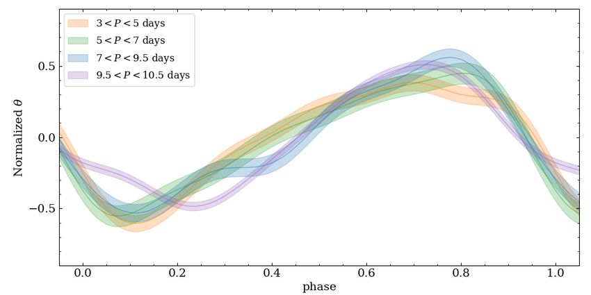
A&A proofs: manuscript no. daSilvaetal2021

Table 1. Sample of 20 calibrating Cepheids with high-resolution spectra covering either a substantial portion or the entire pulsation cycle.

                 Name             αICRS             δICRS        Mode     [Fe/H]lit ± σ    Ref.a    NF     NH    NU     NS    Ntot
                 R TrA         15:19:45.712    −66:29:45.742        0     −0.01 ± 0.03       2       1     14     ...   ...   15
                 T Vul         20:51:28.238    +28:15:01.817        0      0.07 ± 0.10       1      ...    ...    ...   26    26
                 FF Aql        18:58:14.748    +17:21:39.296        1      0.10 ± 0.10       1      ...    ...    ...   27    27
                 S Cru         12:54:21.997    −58:25:50.215        0      0.09 ± 0.04       2      ...    ...    ...   13    13
                 δ Cep         22:29:10.265    +58:24:54.714        0      0.09 ± 0.10       1      ...    ...    ...   18    18
                 Y Sgr         18:21:22.986    −18:51:36.002        0      0.00 ± 0.06       2      ...    20     ...    4    24
                 XX Sgr        18:24:44.500    −16:47:49.820        0      0.06 ± 0.04       2       4     ...    5     3     12
                 η Aql         19:52:28.368    +01:00:20.370       0B      0.24 ± 0.09       2      ...    ...    ...   11    11
                 S Sge         19:56:01.261    +16:38:05.236       0B      0.14 ± 0.10       1      ...    ...    ...   21    21
                 V500 Sco      17:48:37.501    −30:28:33.461       0B     −0.07 ± 0.08       1      ...    ...     4     3     7
                 β Dor         05:33:37.512    −62:29:23.323       0B     −0.03 ± 0.05       2       1     46     ...   ...   47
                 ζ Gem         07:04:06.530    +20:34:13.074       0B      0.16 ± 0.05       2      ...    47     ...   81    128
                 VY Sgr        18:12:04.566    −20:42:14.465       0B      0.25 ± 0.08       2      29     ...     4    ...   33
                 UZ Sct        18:31:22.367    −12:55:43.339       0B      0.11 ± 0.09       2      28     ...     6    ...   34
                 Y Oph         17:52:38.702    −06:08:36.875        0      0.08 ± 0.05       2      ...     8     ...   ...    8
                 RY Sco        17:50:52.345    −33:42:20.411        0      0.01 ± 0.06       1      ...    ...     5     3     8
                 RZ Vel        08:37:01.303    −44:06:52.844        0      0.08 ± 0.06       2       1     11     ...   ...   12
                 V340 Ara      16:45:19.112    −51:20:33.394        0      0.23 ± 0.07       2      26     ...     6    ...   32
                 WZ Sgr        18:16:59.716    −19:04:32.989        0      0.28 ± 0.08       1       1     ...     5     3     9
                 RS Pup        08:13:04.216    −34:34:42.692        0      0.14 ± 0.07       2      ...    15     ...    3    18

Notes. The first four columns give the star name, the right ascension and declination, and the pulsation mode (0: fundamental; 1: first overtone;
0B: fundamental with bump). The Cols. 5 and 6 give the iron abundance from literature and the corresponding references. Columns from 7 to 10
show the number of optical spectra used for each spectrograph: NF : FEROS; NH : HARPS; NU : UVES; NS : STELLA. The last column lists the
total number of spectra per target.
References. (a) 1: Genovali et al. (2014); for T Vul, FF Aql, δ Cep, and S Sge we assumed a typical error of 0.1 dex since they were not provided
by the original authors; 2: Proxauf et al. (2018), from which the uncertainty adopted is the largest value between σ and std.

poor (Romaniello et al. 2021), and those in the Small Magel-               microturbulent velocity (see, e.g., Lemasle et al. 2020; Kovtyukh
lanic Cloud (SMC) a factor of four more metal-poor than so-                2007; Proxauf et al. 2018, and references therein).
lar (Lemasle et al. 2017). Cepheids are intermediate-mass stars                Pioneering investigations based on multiple (from a few to
crossing the instability strip during central helium burning, the          almost two dozen) spectra along the pulsation cycle were pro-
so-called blue loops, and their progenitor mass ranges from ∼3 to          vided more than ten years ago by Luck & Andrievsky (2004),
∼10 M – the exact limit depends on the chemical composition                Kovtyukh et al. (2005), Andrievsky et al. (2005), and Luck et al.
(Bono et al. 2000b; De Somma et al. 2021). Classical Cepheids              (2008), in which they evaluated the variation of the atmospheric
are solid stellar beacons to trace young stellar populations even          parameters and the abundances in both short- and long-period
in the far side of the Galactic thin disk (Minniti et al. 2020,            Cepheids. More recently, we performed a detailed investigation,
2021) and in stellar systems experiencing recent star formation            based on a large dataset of high-resolution spectra, for a sample
events such as dwarf irregulars and star forming galaxies (Nee-            of 14 calibrating Cepheids (Proxauf et al. 2018). In that work,
ley et al. 2021). Their period-luminosity relations (Breuval et al.        the number of spectra per object ranges from five to more than
2020; Ripepi et al. 2020) provide accurate (at the level of ∼1-            120, and the spectra covered a significant portion of the pulsa-
2%) measurements of individual distances. Individual distances             tion cycle. In the same investigation we also used a new and
together with detailed information concerning their elemental              more homogeneous list of Line Depth Ratios (LDR) to estimate
abundances (iron peak, α, neutron capture), provide the unique             the effective temperature directly from the spectra, an approach
opportunity to investigate the radial gradients and, in turn, the re-      that is independent of the photometric properties. The reader in-
cent (t ≤ 200-300 Myr) chemical enrichment history of the thin             terested in a more detailed discussion is referred to Kovtyukh
disk and nearby stellar systems (Romaniello et al. 2008; Lemasle           (2007, and references therein). However, all these investigations
et al. 2013; Genovali et al. 2015; da Silva et al. 2016).                  were hampered by three limitations:
    Furthermore, classical Cepheids are fundamental laborato-
ries for investigating not only the advanced evolutionary phases           a) Line list – We compiled a list of iron lines using line lists
of intermediate-mass stars (Bono et al. 2000a; Neilson et al.                 available in the literature. The sources of atomic transition
2011; Prada Moroni et al. 2012; De Somma et al. 2021), but                    parameters were inhomogeneous, because they did not pass
also for constraining the physical mechanisms driving their vari-             a detailed scrutiny.
ability (Bono et al. 1999; Marconi et al. 2013).                           b) Phase coverage – In spite of the large number of spectra
    Although classical Cepheids are the cross-road of several                 adopted in the spectroscopic analysis, several objects had
recent and long-standing astrophysical problems, we still lack                spectra collected at similar phases and, consequently, they
accurate investigations concerning the variation of their phys-               had a modest phase coverage.
ical properties along the pulsation cycle. The current studies             c) Intrinsic variation – The inhomogeneity of the atomic tran-
are mainly based on both optical and near-infrared (NIR) light                sition parameters introduces uncertainties in the spectro-
curves, but we still lack detailed spectroscopic analysis concern-            scopic surface gravity and in the microturbulent velocity.
ing the variation of effective temperature, surface gravity, and              This caused an increase in the standard deviation at fixed
Article number, page 2 of 31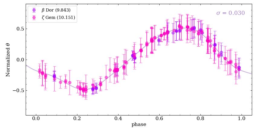
R. da Silva et al.: A new and homogeneous metallicity scale for Galactic classical Cepheids

Fig. 1. Examples of high-resolution spectra for the stars β Dor and ζ Gem in different pulsation phases (values on the right side of each panel).
The vertical red lines indicate the position in the rest-frame wavelength of atomic lines either only used for the abundance determination or also
adopted by the LDR method. For the sake of clarity the continuum of each spectrum was shifted to arbitrary levels.

    pulsation phase, and in turn, some limitation in the analysis         velocity and photometric data used. In Sect. 5 we explain how we
    of their variation along the pulsation cycle.                         derived the atmospheric parameters and their variation along the
                                                                          pulsation cycle. The iron and α-element abundances and their
     To overcome these limitations, the current investigation is          variation along the pulsation cycle are discussed in Sect. 6. A
based on a new approach including five steps: i) We updated the           summary of the results and some final remarks concerning this
atomic transition parameters of our line lists with more recent           project are given in Sect. 7.
and accurate laboratory measurements available in the literature;
ii) We collected new high signal-to-noise ratio (S/N) and high-
resolution spectra for our sample of calibrating Cepheids, and we         2. Spectroscopic datasets
also performed a detailed search for similar quality spectra avail-
able in online science archives. This translates into an increase in      The spectroscopic datasets analyzed in the current paper are
the number of calibrating Cepheids by almost 50% (from 14 to              spectra collected using several different instruments. Three of
20). Moreover, we also added new spectra to Cepheids already              them are mounted on telescopes of the European Southern Ob-
included in the former sample. The current sample includes 19             servatory (ESO): the High Accuracy Radial velocity Planet
stars pulsating in the fundamental mode and, for the first time           Searcher (HARPS; Mayor et al. 2003) at the 3.6 m, the Fiber-
used by us as a calibrating Cepheid, one star (FF Aql) pulsat-            fed Extended Range Optical Spectrograph (FEROS; Kaufer et al.
ing in the first overtone mode, and their metallicities range from        1999) at the 2.2 m MPG/ESO, and the Ultraviolet and Visual
−0.08 (β Dor) to 0.19 dex (VY Sgr); iii) We performed a detailed          Echelle Spectrograph (UVES; Dekker et al. 2000) at the Very
visual check of hundreds of lines along the pulsation cycle to            Large Telescope. The other instrument is the STELLA Echelle
create a new homogeneous line list. Special attention was paid            Spectrograph (SES; Strassmeier et al. 2004, 2010) located at the
in the identification of lines showing blends (or poor definition         Izãna Observatory on Tenerife in the Canary islands.
of the continuum), or having any correlation with the effective               The spectral resolution of the quoted spectrographs for the
temperature (due to possible NLTE effects) or with the equiva-            instrument settings used are R∼40 000 (UVES), R∼115 000
lent widths (due to saturated lines), or presenting any systematic        (HARPS), R∼48 000 (FEROS), and R∼55 000 (STELLA). For
over- or under-abundance; iv) We improved the algorithm that              details on the wavelength ranges of our spectra we refer the
we use for the estimate of the atmospheric parameters, and in             reader to Sect. 2 of the papers Proxauf et al. (2018) and Crestani
turn, for the estimate of the elemental abundances; v) In addition        et al. (2021).
to the atmospheric parameters and iron abundances, the current                The entire spectroscopic sample includes reduced spectra
study also includes the abundances of five α elements: Mg, Si,            downloaded from the ESO and the STELLA archives, for a total
S, Ca, and Ti.                                                            of 1383 spectra of 285 stars: 199 HARPS spectra of 9 stars, 419
     We notice that the star AV Sgr, which was one of the cali-           FEROS spectra of 151 stars, 450 STELLA spectra of 68 stars,
brating Cepheids in Proxauf et al. (2018), is not included in the         and 315 UVES spectra of 123 stars. Their S/N ranges from a
current work. The reason is that, after the revision of the Fe line       few tens to more than 400 (about 70% of our spectra have S/N
list, we were not able to derive accurate estimates of the atmo-          of at least 100). From this sample we selected the spectra of 20
spheric parameters for many of the spectra of this variable. The          targets that cover either a significant part (about half or more)
number of spectra with accurate measurements was not enough               or the entire pulsation cycle. From now on we refer to this sub-
to provide a good coverage of the pulsation cycle, and therefore,         sample as our sample of 20 calibrating Cepheids. Details on the
it was removed from the list of calibrating Cepheids. The pa-             number of spectra are given in Table 1.
rameters published in our previous paper can still be used, but
keeping in mind that they are based on a different version of the         3. Data reduction and analysis
line list.
     The structure of the paper is the following: in Sect. 2 we           As mentioned in Proxauf et al. (2018), the spectra from UVES
discuss the spectroscopic dataset and provide detailed informa-           and HARPS (Phase 3) were already pre-reduced (i.e., reduced
tion concerning the current sample of calibrating Cepheids. In            up to the wavelength calibration step) by their own pipeline. As
Sect. 3 we discuss the data reduction process and introduce the           previously done, the FEROS spectra were reduced using a mod-
atomic line lists used. Sect. 4 includes a description of the radial-     ified version of the Data Reduction System (DRS) pipeline. A
                                                                                                                     Article number, page 3 of 31
A&A proofs: manuscript no. daSilvaetal2021

Fig. 2. Iron abundances as a function of the pulsation phase, effective temperature, and equivalent width. These are examples of good lines that
were kept in our initial line list for HARPS (green circles), FEROS (blue triangle), and STELLA (red stars) spectra of β Dor and ζ Gem. The
hatched regions around the dashed lines indicate the 1-σ uncertainty around the mean.

few tens of FEROS spectra collected before 2004, which initially         Table 2. Excerpt from the list of Fe i and Fe ii atomic lines.
could not be reduced, were later on reduced and delivered by one
of the Phase 3 Data Releases (DR3 and DR3.1). However, they                                                                   Quality
are all low-quality spectra that were not included in our analysis.            λ [Å]       Species     ξ [eV]      log g f                Ref.
                                                                                                                               flag
    After the pre-reduction steps, all the selected spectra were
normalized to the continuum using the Image Reduction and                    3763.789        Fe i       0.989     −0.220          1         1
Analysis Facility (IRAF 1 ) by fitting cubic spline functions to             3787.880        Fe i       1.010     −0.840          1         1
a set of continuum windows. An exception is the case of the                     ...           ...         ...       ...          ...
STELLA spectra, which were reduced by a dedicated pipeline                   7655.488        Fe ii      3.892     −3.560          1         2
(Weber et al. 2012) based on IRAF routines and that includes                 7711.724        Fe ii      3.903     −2.500          1         2
several reduction steps up to the continuum normalization.
                                                                         Notes. The quality flag column indicates if the line was used (1) or not
    For more details about the quality of the spectra we refer the       used (0) in the current study. The complete table is available at the CDS.
reader to Sect. 3 of Proxauf et al. (2018), which also includes a
figure (their Fig. 1) showing a few examples of HARPS, FEROS,            References. 1: O’Brian et al. (1991); 2: Meléndez & Barbuy (2009); 3:
                                                                         NIST: Kramida et al. (2020).
UVES, and STELLA spectra of different metallicities and S/N.
In our Fig. 1, we plot an example of HARPS spectra for β Dor
and of STELLA spectra for ζ Gem in different pulsation phases,           Table 3. The same as in Table 2 but showing an excerpt of atomic lines
showing how the profile of the absorption lines may change (in           from the list of α elements.
depth and in shape) along the pulsation cycle. Studies of line
asymmetry changes over the pulsation cycle of Cepheid stars                                                                   Quality
were also reported by Nardetto et al. (2006) and Nardetto et al.               λ [Å]       Species     ξ [eV]      log g f                Ref.
                                                                                                                               flag
(2008), in a series of papers on high-resolution spectroscopy, for
                                                                             3829.355       Mg i        2.709     −0.227          0         3
Fe i and Hα lines in the optical and, more recently, by Nardetto
                                                                             4571.096       Mg i        0.000     −5.620          1         3
et al. (2018) for the Na i line at 2208.969 nm.
                                                                                ...          ...          ...       ...          ...
                                                                             6606.956       Ti ii       2.061     −2.790          1         3
3.1. Line lists and equivalent widths                                        7214.729       Ti ii       2.590     −1.750          1         3
Similarly to what we did in our previous works, here we use
three different line lists:
                                                                             The Cepheids variables are bright stars and thus we have
a) one containing atomic lines of N, Si, S, Ca, Ti, V, Cr, Mn,           at our disposal very high S/N, broad wavelength range spectra.
   Fe, Co, and Ni, created from a combination of four line lists         The precision of the atmospheric parameters and of the chemi-
   received from V. Kovtyukh (for a total of 153 atomic lines).          cal abundances, however, depends not only on the quality of the
   These lines are used to derive the effective temperature (T eff )     spectra, but also on the quality of the adopted line list. With this
   of our sample stars according to the procedure described in           in mind, a large portion of the present work was dedicated to
   Sect. 4.2 of Proxauf et al. (2018);                                   finding the best atomic transitions for iron and α elements that
b) one containing 424 Fe i and 97 Fe ii lines, created from              can be detected in Cepheids. In practice, this means i) collecting
   a combination of lines from Genovali et al. (2013) with               the most precise transition parameters, ii) removing absorption
   lines from the Gaia-ESO Survey (GES, Gilmore et al. 2012;             lines that are blended with other lines, and iii) eliminating lines
   Randich et al. 2013). It is used as a reference line list in the      that for any reason deviate significantly from the average value
   determination of both the stellar surface gravity (log g), as         for their chemical species, or that display a dependency on any
   described in Sect. 5.1, and the stellar metallicity, as discussed     quantity that changes across the pulsation cycle, such as the ef-
   in Sect. 6;                                                           fective temperature.
c) one containing lines of α elements (Mg: 9 lines; Si: 11 lines;            In order to address the first point, we departed from a list
   S: 1 line; Ca: 36 lines; and Ti: 72 lines), based on line lists       of hundreds of atomic transitions for iron and α elements com-
   from For & Sneden (2010), Venn et al. (2012), Lemasle et al.          monly employed in the literature. We updated their transition
   (2013), and McWilliam et al. (2013, and references therein).          parameters whenever possible with the updated laboratory mea-
1
  The IRAF package is distributed by the National Optical Astronomy      surements from Ruffoni et al. (2014), Den Hartog et al. (2014),
Observatories (NOAO), USA.                                               and Belmonte et al. (2017) for Fe i, Den Hartog et al. (2019) for
Article number, page 4 of 31
R. da Silva et al.: A new and homogeneous metallicity scale for Galactic classical Cepheids

                                                                          Fig. 4. Photometric amplitude as a function of the logarithmic period
                                                                          (Bailey diagram). Our calibrating Cepheids are represented by colored
                                                                          symbols whereas the Cepheids from literature (Luck et al. 2011; Luck
                                                                          & Lambert 2011; Lemasle et al. 2013; Yong et al. 2006) are shown in
                                                                          light gray circles.

                                                                          shown in the same tables with quality flag 0, were measured only
                                                                          for comparison purposes.
                                                                               An example of a good Fe line is shown in Fig. 2 for β Dor
                                                                          and ζ Gem. Examples and a description of the typical behavior
Fig. 3. Top: RV curve of the fundamental pulsator S Cru. The red solid    of irregular (less reliable) lines are found in the Appendix A,
line displays the PLOESS fit to the RV curve. The horizontal red dashed   in the plots of Figs. A.1-A.5. These same irregular lines, how-
and dotted lines display the mean RV (hRVi) and its uncertainty. The      ever, might provide good results for other stars, for instance, of
vertical red dotted line displays the phase where RV equals hRVi on the   different spectral types, or having spectra of different quality or
rising branch. The name, hRVi, period and reference epoch are labelled.
Bottom: same as in the top panel but for the V-band light curve, its
                                                                          different resolution. This is the reason why we preferred to ex-
PLOESS fit and its mean value. We note that, within the uncertainty,      clude some lines only for this particular analysis, and keep the
the light curve is co-phased with the RV curve.                           initial line lists as they are to be used in future studies. It is worth
                                                                          mentioning that we only excluded lines that were clearly having
                                                                          problems in most of the stars in our sample.
Fe ii, Lawler et al. (2013) for Ti i, and Wood et al. (2013) for Ti ii.
We also made ample use of the astrophysical, but homogeneous              4. Radial velocity and photometric data
and precise compilation of Meléndez & Barbuy (2009) for Fe ii.
For the remaining lines, we adopted the transition parameters             The radial velocity (RV) measurements for our sample were
collected and updated by the National Institute of Standards and          done using the following methods: i) for HARPS and UVES
Technology (NIST) Atomic Spectra Database (Kramida et al.                 spectra, we used IRAF packages to cross-correlate the target
2020). If a line is not available in any of these sources, it is elim-    spectrum with a solar template spectrum (Solar flux atlas from
inated from the preliminary list and not used for the computation         296 to 1300 nm, Kurucz et al. 1984) degraded to the UVES res-
of atmospheric parameters nor chemical abundances.                        olution; ii) for FEROS spectra we adopted the RVs derived by
    With this preliminary list at hand, we addressed the second           ARES, the routine we used for the equivalent width measure-
point mentioned above by removing any blended lines, using                ments (see Sect. 3.1); iii) the STELLA radial velocities are writ-
as reference the Solar spectrum table by Moore et al. (1966)              ten in the header of the FITS files and they are based on cross-
and synthetic spectra. Then we measured their equivalent width            correlations with a template spectrum, performed by a dedicated
(EW) using the Automatic Routine for line Equivalent widths in            reduction pipeline also using IRAF. In case of the Cepheids, a
stellar Spectra (ARES, Sousa et al. 2007, 2015).                          G-type dwarf template is used.
                                                                              The uncertainties adopted for these RV estimates depend on
    Finally, we addressed the third point by removing deviant             the method used: for HARPS, UVES, and STELLA spectra, the
lines. In a first iteration, we estimated initial values for the atmo-    uncertainties are estimated by IRAF during the cross-correlation;
spheric parameters and the chemical abundances. Lines are con-            for FEROS spectra, they are estimated by ARES using spectral
sidered deviant if they result in abundances diverging by at least        windows free of lines. Typical values for our HARPS, UVES,
3 σ from the mean for a given element, or if their behavior across        and FEROS spectra range from a few m/s in the best cases to
the pulsation cycle is irregular. This latter situation is investi-       a few km s−1 , depending on the spectral type. For the STELLA
gated by plotting all line-by-line measurements for each chemi-           spectra, we adopted an uncertainty of 0.2 km s−1 . This is a con-
cal species and individual exposure of our calibrating stars ver-         servative estimate considering that typical formal errors for high
sus phase, effective temperature, and equivalent width, and re-           S/N spectra of Cepheids stars is about 50 m s−1 and that the
moving lines that show strong trends in any of those planes. The          RV zero point for this spectrograph has RMS variations of 30
calibrating stars mostly used are those with the largest number           to 150 m s−1 over two years. The RV estimates and the corre-
of individual spectra covering the whole pulsation cycle, such as         sponding uncertainties for our sample of calibrating Cepheids
β Dor, ζ Gem, and FF Aql.                                                 are listed in Table 4.
    The final clean lists, shown in Tables 2 and 3 with quality flag          In addition to our own RV measurements, we adopted litera-
1, were used to compute the final atmospheric parameters and              ture RV curves and light curves to provide accurate ephemerides,
chemical abundances for the whole sample. The remaining lines,            meaning reference epoch (T 0 ) plus pulsation period (P) for these
                                                                                                                    Article number, page 5 of 31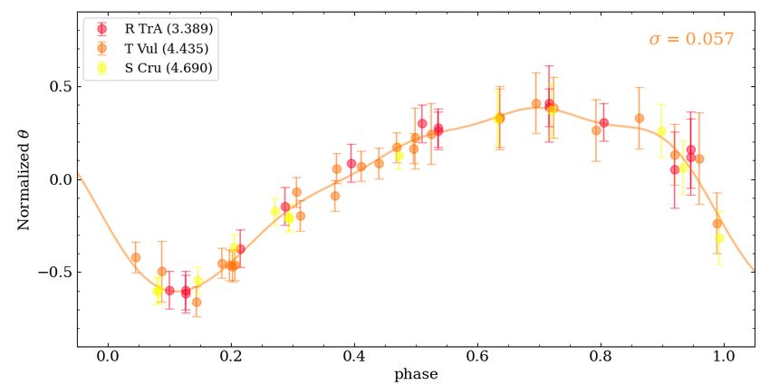
A&A proofs: manuscript no. daSilvaetal2021

Table 4. Excerpt from the list of atmospheric parameters, Fe abundances, and radial velocities for each spectrum of the 20 calibrating Cepheids.

                                        MJD          T eff ± σ                υt                                                               RV ± σ
               Name       Dataset                                log g     [km s−1 ]       Fe i ± σ      NFe i      Fe ii ± σ       NFe ii
                                        [d]             [K]                                                                                    [km s−1 ]
               R TrA     HARPS      53150.1353086   5918 ± 154   2.3         3.5         −0.02 ± 0.09     86     −0.03 ± 0.03         7       2.57 ± 1.38
               R TrA     HARPS      53150.1453265   5892 ± 128   2.3         3.6         −0.04 ± 0.09     81     −0.05 ± 0.02         8       2.40 ± 1.37
               ...          ...           ...            ...     ...          ...              ...        ...          ...           ...           ...
               RS Pup    STELLA     57708.2167938   5508 ± 98    0.9         3.4          0.12 ± 0.11    107      0.12 ± 0.15         7       7.40 ± 0.20
               RS Pup    STELLA     57713.2628277   5298 ± 111   ...         ...               ...        ...          ...           ...     16.25 ± 0.20

Notes. The first three columns give the target name, spectroscopic dataset, and Modified Julian Date at which the spectrum was collected.
Columns 4, 5, and 6 give, respectively, the effective temperature and its standard deviation, surface gravity, and microturbulent velocity. The
Cols. 7-8 and 9-10 list both the Fe i and Fe ii abundances derived from individual lines together with the standard deviations and the number of
lines used (for the Fe ii abundances, a minimal uncertainty of 0.11 dex was adopt when computing the mean abundances, as described in the text).
The last column gives the radial velocities with their uncertainties. The complete table is available at the CDS.

Table 5. Photometric and radial-velocity parameters for our sample of 20 calibrating Cepheids.

                          V             ∆V                γ                ∆RV              LC             Period           T 0 − 2 400 000         Ephemerides
     Name                                               [km/s]
                        [mag]          [mag]                              [km/s]          sourcea          [days]                [days]               sourceb
     R TrA            6.66 ± 0.02   0.56 ± 0.02     –12.44 ± 2.54        28.1 ± 2.2           1          3.3892582              44 423.59377                1
     T Vul            5.75 ± 0.03   0.64 ± 0.04       0.85 ± 0.11        34.5 ± 3.5           1          4.435462               57 632.18950                0
                                                                                                                                50 735.20310                2
     FF Aql           5.19 ± 0.01   0.33 ± 0.03     –11.36 ± 0.10        16.1 ± 1.5           2          4.470916               56 888.66207                0
     S Cru            6.60 ± 0.02   0.73 ± 0.03      –4.70 ± 0.28        33.8 ± 4.3           1          4.68973                55 279.67331                0
     δ Cep            3.94 ± 0.01   0.84 ± 0.04     –16.32 ± 0.20        38.9 ± 4.9           1          5.3663                 56 917.54900                0
     Y Sgr            5.74 ± 0.02   0.72 ± 0.03      –2.84 ± 3.02        34.2 ± 3.0           1          5.7733866              54 946.78504                1
     XX Sgr           8.86 ± 0.02   0.87 ± 0.04      12.30 ± 0.46        41.6 ± 1.2           1          6.4243013              54 946.67631                1
     η Aql            3.89 ± 0.02   0.78 ± 0.03     –14.47 ± 0.63        42.1 ± 2.2           1          7.1768572              50 724.43545                1
     S Sge            5.61 ± 0.03   0.72 ± 0.03     –16.40 ± 0.25        39.3 ± 4.7           1          8.3445707              57 636.28926                0
                                                                                                                                48 746.52000                3
                                                                                                         8.3823514              50 339.17710                4
     V500 Sco         8.74 ± 0.01   0.71 ± 0.05      –7.61 ± 3.37        32.2 ± 5.4           1          9.317                  44 789.61621                1
     β Dor            5.25 ± 0.01   0.63 ± 0.06       8.17 ± 0.11        32.9 ± 2.3           2          9.84308                53 284.79472                0
                                                                                                         9.8527371              41 149.27150                4
     ζ Gem         3.89 ± 0.03      0.49 ± 0.03       6.78 ± 0.42        26.5 ± 1.0           1         10.149816               54 805.78476                1
     VY Sgr       11.46 ± 0.02      1.14 ± 0.05      14.23 ± 1.58        50.4 ± 4.4           1         13.55845                54 171.32722                1
     UZ Sct       11.25 ± 0.03      0.75 ± 0.05      39.52 ± 0.18        44.7 ± 3.5           0         14.744162               56 171.62381                0
     Y Oph         6.15 ± 0.02      0.49 ± 0.03      –7.56 ± 2.01        16.5 ± 2.0           1         17.12633896             53 209.96732                1
     RY Sco        8.02 ± 0.02      0.83 ± 0.03     –17.73 ± 2.02        30.1 ± 3.0           1         20.321538               45 077.36644                1
     RZ Vel        7.09 ± 0.04      1.17 ± 0.05      24.11 ± 4.52        54.6 ± 5.4           1         20.399727               50 776.13608                1
     V340 Ara     10.20 ± 0.06      1.08 ± 0.07     –76.25 ± 4.19        47.7 ± 9.3           1         20.811386               56 138.97597                0
     WZ Sgr        8.03 ± 0.03      1.08 ± 0.05     –17.78 ± 1.17        54.2 ± 2.9           1         21.849708               50 691.28534                1
     RS Pup        6.99 ± 0.03      1.11 ± 0.04      25.80 ± 1.91        48.5 ± 2.1           1         41.488634               53 092.94483                1

Notes. From left to right the columns give the star name, the mean magnitude in visual bands, the magnitude amplitude, the mean radial velocity,
the RV amplitude, the light curve source, the pulsation period and zero-phase reference epoch of mean magnitude (or mean radial velocity), and
the Ephemerides source. For the variables VY Sgr, RZ Vel, and WZ Sgr, our RV measurements and those by Groenewegen (2008, and references
therein) show a shift in phase of −0.05, +0.03, and −0.03, respectively. To co-phase the two datasets, the latter sample of radial velocities plotted
in Fig. B.1 were shifted.
References. (a) 0: ASAS-SN (Shappee et al. 2014; Kochanek et al. 2017); 1: Groenewegen (2008, and references therein); 2: Pel (1976). (b) 0:
Period and T 0 derived from our own radial velocity curves; 1: Period and T 0 derived from the radial velocities by Groenewegen (2008, and
references therein); 2: T 0 derived from the light curve; 3: T 0 derived from the radial velocities by Groenewegen (2008, and references therein); 4:
Period and T 0 derived from the light curve.

variables. More specifically, we collected RV curves and V-band                     et al. (2015), we have been promoting the use of another refer-
light curves from Pel (1976) and Groenewegen (2008, and ref-                        ence for both Cepheids and RR Lyrae, that is, the epoch of the
                                                                                                                                                    opt
erences therein). For UZ Sct, we adopted the V-band light curve                     mean magnitude on the rising branch of the light curve (T mean )
from the All-Sky Automated Survey for Supernovae (ASAS-SN,                          or, equivalently, the epoch of mean velocity on the decreasing
Shappee et al. 2014; Kochanek et al. 2017) because it is the only                                                RV
                                                                                    branch of the RV curve (T mean  ). See Fig. 3 for a visualization of
well-sampled light curve that can be co-phased with our RV time                     this reference epoch on both the light and RV curves. A detailed
series.                                                                                                    opt
                                                                                    procedure to derive T mean is described in Braga et al. (2021).
    We estimated the pulsation periods of our targets by us-                                                 opt
                                                                                    The advantages of the T mean reference epoch over T max are well-
ing our own interactive method (Braga et al. 2016) based on                         explained in Inno et al. (2015) and quantitatively discussed in
the Lomb-Scargle periodogram (Scargle 1982). Historically, the                      Braga et al. (2021).
most commonly used T 0 is the time of maximum light (T max ),
which matches the time of minimum velocity. Starting from Inno
Article number, page 6 of 31
R. da Silva et al.: A new and homogeneous metallicity scale for Galactic classical Cepheids
Table 6. Mean atmospheric parameters derived for the 20 calibrating Cepheids.
hT eff i ± σ Nspec hυt i ± σ
Name hθi ± σ ∆θ ± σ hlog gi ± σ [Fe i/H] ± σ [Fe ii/H] ± σ [Fe/H] ± σ (std) Nspec
[K] (T eff ) [km s−1 ]
R TrA 6035 ± 25 0.840 ± 0.010 0.098 ± 0.016 15 2.01 ± 0.08 3.23 ± 0.13 −0.03 ± 0.02 −0.03 ± 0.03 −0.03 ± 0.02 (0.02) 15
T Vul 5934 ± 20 0.855 ± 0.010 0.122 ± 0.024 26 1.43 ± 0.06 3.07 ± 0.10 −0.04 ± 0.02 −0.03 ± 0.02 −0.04 ± 0.02 (0.05) 26
FF Aql 6182 ± 18 0.820 ± 0.010 0.058 ± 0.012 27 1.35 ± 0.06 3.03 ± 0.10 0.05 ± 0.02 0.05 ± 0.03 0.05 ± 0.02 (0.05) 27
S Cru 6018 ± 20 0.862 ± 0.010 0.140 ± 0.028 13 1.57 ± 0.08 3.01 ± 0.14 −0.03 ± 0.02 −0.01 ± 0.03 −0.02 ± 0.02 (0.07) 13
δ Cep 5905 ± 22 0.862 ± 0.010 0.154 ± 0.022 18 1.42 ± 0.07 3.08 ± 0.12 0.06 ± 0.02 0.05 ± 0.03 0.05 ± 0.02 (0.05) 18
Y Sgr 5914 ± 25 0.877 ± 0.020 0.128 ± 0.027 24 1.58 ± 0.06 3.48 ± 0.10 0.03 ± 0.02 0.02 ± 0.03 0.02 ± 0.02 (0.08) 23
XX Sgr 5884 ± 29 0.855 ± 0.010 0.151 ± 0.031 12 1.25 ± 0.09 2.92 ± 0.14 −0.01 ± 0.03 −0.01 ± 0.04 −0.01 ± 0.02 (0.05) 12
η Aql 5480 ± 40 0.891 ± 0.030 0.113 ± 0.035 11 1.16 ± 0.09 3.43 ± 0.15 0.09 ± 0.04 0.08 ± 0.04 0.09 ± 0.03 (0.10) 11
S Sge 5777 ± 21 0.883 ± 0.012 0.134 ± 0.019 21 1.20 ± 0.07 3.13 ± 0.11 0.10 ± 0.02 0.09 ± 0.03 0.09 ± 0.02 (0.05) 21
V500 Sco 5797 ± 32 0.850 ± 0.053 7 1.21 ± 0.11 3.04 ± 0.19 −0.03 ± 0.04 −0.03 ± 0.04 −0.03 ± 0.03 (0.02) 7
β Dor 5552 ± 13 0.903 ± 0.020 0.132 ± 0.023 47 1.15 ± 0.04 3.31 ± 0.07 −0.07 ± 0.01 −0.08 ± 0.02 −0.08 ± 0.01 (0.04) 47
ζ Gem 5500 ± 8 0.914 ± 0.020 0.100 ± 0.011 128 1.14 ± 0.03 3.32 ± 0.04 0.02 ± 0.01 0.01 ± 0.01 0.01 ± 0.01 (0.06) 128
VY Sgr 5343 ± 27 0.954 ± 0.020 0.214 ± 0.048 24 1.09 ± 0.08 3.38 ± 0.13 0.19 ± 0.04 0.18 ± 0.04 0.19 ± 0.03 (0.11) 14
UZ Sct 5113 ± 25 0.979 ± 0.045 25 0.87 ± 0.09 3.35 ± 0.16 0.14 ± 0.04 0.10 ± 0.05 0.12 ± 0.03 (0.07) 10
Y Oph 5609 ± 33 0.900 ± 0.013 8 1.20 ± 0.11 3.79 ± 0.18 −0.05 ± 0.04 −0.05 ± 0.05 −0.05 ± 0.03 (0.02) 8
RY Sco 5743 ± 36 0.886 ± 0.071 8 0.99 ± 0.11 3.69 ± 0.18 0.05 ± 0.04 0.04 ± 0.04 0.04 ± 0.03 (0.07) 8
RZ Vel 5483 ± 29 0.919 ± 0.020 0.232 ± 0.037 12 1.02 ± 0.09 4.35 ± 0.15 0.04 ± 0.02 0.03 ± 0.05 0.03 ± 0.02 (0.11) 11
V340 Ara 5170 ± 26 0.933 ± 0.057 32 1.10 ± 0.09 4.60 ± 0.16 0.12 ± 0.04 0.08 ± 0.05 0.10 ± 0.03 (0.09) 10
WZ Sgr 5411 ± 33 0.924 ± 0.067 9 0.89 ± 0.11 3.77 ± 0.19 0.13 ± 0.04 0.11 ± 0.05 0.12 ± 0.03 (0.07) 7
RS Pup 5432 ± 25 0.901 ± 0.020 0.195 ± 0.032 18 0.81 ± 0.07 3.74 ± 0.12 0.07 ± 0.02 0.09 ± 0.03 0.08 ± 0.02 (0.06) 16
Notes. Columns from 1 to 5 give, respectively, the star name, the mean effective temperature and mean θ, the θ amplitude (see Section 5.2), and the
number of spectra used to compute these mean values. Columns from 6 to 9 lists the surface gravity, microturbulent velocity, and iron abundances
from neutral and ionized lines. These are the weighted mean values and their standard errors computed from the individual measurements listed
in Table 4. Column 10 gives the weighted iron abundance and its standard error, calculated from Cols. 8 and 9. The standard deviation calculated
using all individual measurements from both Fe i and Fe ii lines is also shown within parentheses. The last column gives the number of spectra
used to derive log g, υt , and the iron abundances.
The light and radial-velocity curves for all the sample stars 5. Atmospheric parameters and effective
are shown in the Appendix B, in Fig. B.1. The estimated temperature curve templates
ephemerides of our targets are listed in Table 5 together with
the mean magnitudes and magnitude amplitudes in the visual 5.1. Effective temperature, surface gravity, and
band, and the mean radial velocities and RV amplitudes. We no- microturbulent velocity
ticed that for the stars VY Sgr, RZ Vel, and WZ Sgr, for which The approach we adopted to estimate the atmospheric param-
the new period and T 0 values are based on the radial velocities eters (i.e., the effective temperature, the surface gravity, and
derived by Groenewegen (2008, and references therein), the new the microturbulent velocity) was already discussed in detail by
ephemerides caused a shift in phase between the two datasets Proxauf et al. (2018). Here we only recap the key points. The
shown in Fig. B.1. To overcome this problem, we applied a shift T eff along the pulsation cycle was estimated by using the LDR
of −0.05, +0.03, and −0.03, respectively, to the literature data method, which relies on the correlation between the line depth
plotted in these panels. ratios of pairs of absorption lines in the spectra of different stars
and the effective temperature of the same stars. The surface grav-
ity was derived through the ionization equilibrium of Fe i and
Fe ii lines, and the microturbulent velocity was obtained by mini-
mizing the dependence of the abundances provided by single Fe i
Figure 4 shows the distribution of the current calibrating lines on their EWs. During this procedure, the effective tempera-
Cepheids (colored symbols), together with Galactic Cepheids ture was kept fixed, whereas log g and ξ were iteratively changed
available in the literature (light gray circles), in the so-called until convergence. The metallicity used as input by our algorithm
Bailey diagram (luminosity amplitude as a function of the loga- is updated in each step, and the adopted value is [Fe i/H], which
rithmic period). The plotted data display the classical "V" shape is the mean iron abundances provided by individual Fe i lines.
in which the local minimum around ten days is mainly caused The estimates of T eff , log g, and ξ for the individual spectrum
by the Hertzsprung progression (Bono et al. 2000b). By having of our sample are listed in Table 4. The uncertainties on T eff are
a look also at Fig. B.1, we see a subgroup of classical Cepheids the standard deviation calculated using the LDR method, that is,
showing a well defined bump on the light curve. The phase of from the effective temperatures provided by the individual pairs
such bumps moves from the decreasing branch for periods be- of lines. The uncertainties on the individual estimates of log g
tween ∼6 and ∼9 days, passing across the maximum for periods and ξ are assumed to be of the order of 0.3 dex and 0.5 km s−1 ,
between ∼9 and ∼12 days, and along the rising branch for peri- respectively (see Genovali et al. 2014, for a detailed discussion).
ods between ∼12 and ∼16 days. At the center of the Hertzsprung The weighted mean values of the atmospheric parameters are
progression (P∼10 days) the light curve is flat topped and the lu- listed in Table 6 together with the corresponding standard errors
minosity amplitude attains a well defined minimum (Bono et al. calculated for each calibrating Cepheid.
2000b, 2002). These variables are called Bump Cepheids for In the Appendix B, Figs. B.2, B.3, and B.4 show the variation
avoiding to be mixed-up with the Beat Cepheids, that is, clas- of the atmospheric parameters along the pulsation cycle. To pro-
sical Cepheids pulsating simultaneously in two or more modes. vide a quantitative estimate of the differences between the cur-
The calibrating Cepheids cover both the short- and the long- rent approach and our previous measurements, we fitted Fourier
period range, and in particular, the current sample includes seven series to the effective temperature, surface gravity, and micro-
Cepheids across the Hertzsprung progression. turbulent velocity curves in order to evaluate their amplitudes,
Article number, page 7 of 31A&A proofs: manuscript no. daSilvaetal2021
Fig. 6. Normalized θ (5040/T eff ) as a function of the pulsation phase
showing the fits of the Fourier series to the data of Fig. 5. The shaded
areas display the 1-σ standard deviation.
Table 7. Coefficients of the Fourier series fitted to the data shown in
Fig. 5 for different bins of pulsation period.
3R. da Silva et al.: A new and homogeneous metallicity scale for Galactic classical Cepheids
Fig. 7. Distribution of standard deviations computed from individual
abundances of Fe i and Fe ii lines. The panels show the histogram for
spectra of stars in common with Proxauf et al. (2018).
5.2. Effective temperature curve templates Fig. 8. Atmospheric parameters differences for stars in common with
Proxauf et al. (2018). Each panel shows our previous determinations
By taking advantage of the substantial phase coverage of our subtracted by the current values.
sample of calibrating Cepheids, we used the effective tempera-
ture measurements to compute new templates for different bins
of pulsation periods. However, instead of using the T eff curves riod bins, they are either not as well sampled as the data for the
directly, we preferred to provide templates for the theta param- other Cepheids, or the theta curves do not overlap well because
eter — defined as θ = 5040/T eff — given its linear dependency the number of measurements is too limited. More accurate and
on the Cousins R-I color index (Taylor 1994). homogeneous data are required to overcome this limitation.
The approach is similar to the NIR light-curve templates pro-
In order to allow the reader to use these curve templates to
vided by Inno et al. (2015): first, we adopted the ephemerides in
derive the mean effective temperature by using the ephemerides,
Table 5 to fold the θ curves (θCs). Subsequently, we normal-
the luminosity amplitude (∆V), and a single spectroscopic mea-
ized the folded θCs by subtracting their average and dividing by
surement of the T eff , we also provide a linear relation between
their amplitudes. Our θCs are well sampled, meaning that we
∆V and ∆θ:
have enough phase points to separate the Cepheids into differ-
ent period bins and to provide analytical relations for the θ curve
templates in each bin. We adopted the same period thresholds ∆θ = (0.184 ± 0.014)∆V + (0.000 ± 0.011); (σ = 0.013) (1)
introduced by Inno et al. (2015). Therefore, based on their Ta-
ble 1, we generated four cumulative and normalized theta curves
for the bins 2 (3-5 days, three Cepheids), 3 (5-7 days, three The estimate of the ∆θ amplitude has to be applied to the normal-
Cepheids), 4 (7-9.5 days, two Cepheids), and 5 (9.5-10.5 days, ized template as a multiplicative factor. Only after this rescaling
two Cepheids). By adopting the same period bins we are able operation the template can be anchored to the empirical data and
to provide θC templates that are homogeneous with those from used to derive the mean T eff .
the NIR light curves. The reader interested in a more detailed Optical and NIR light curves of the calibrating Cepheids,
and quantitative discussion concerning the use of cumulative and together with effective temperature and radial velocity curves,
normalized curves to derive the analytical fits, together with the will be adopted by our group to perform a detailed comparison
adopted thresholds for the different period bins, is referred to with nonlinear, convective hydrodynamical models of classical
Inno et al. (2015). Cepheids. Dating back to Natale et al. (2008) it has been found
The four normalized θ curves are separately shown in Fig. 5, that the simultaneous fit of both luminosity and radial-velocity
and in Fig. 6 we compare the Fourier series fitted to the data of variations provides solid constraints on the physical assumptions
each bin. The corresponding coefficients of the fitted functions adopted to build pulsation models (Marconi et al. 2013). More-
are listed in Table 7. The separation of the Cepheids into differ- over, the use of the effective temperature curves (shapes and am-
ent period bins is a mandatory step because not only the ampli- plitudes), covering a broad range of pulsation periods, brings for-
tude of the theta curves (listed in Table 6), but also their shape ward the opportunity to constrain, on a quantitative basis, the
changes with period (as shown in Figs. 5 and 6). Although we do efficiency of the convective transport over the entire pulsation
have data for Cepheids with periods outside of the selected pe- cycle.
Article number, page 9 of 31A&A proofs: manuscript no. daSilvaetal2021
Table 8. Excerpt from the list of abundances of α elements for each spectrum of the 20 calibrating Cepheids.
MJD
Name Dataset [Mg/H] ± σ NMg ... Ti i ± σ NTi i Ti ii ± σ NTi ii [Ti/H] ± σ
[d]
R TrA HARPS 53150.1453265 0.20 ± 0.11 1 ... −0.21 ± 0.15 8 0.05 ± 0.10 2 −0.12 ± 0.19
R TrA HARPS 53150.1353086 0.17 ± 0.11 1 ... −0.17 ± 0.27 12 0.01 ± 0.10 3 −0.14 ± 0.25
... ... ... ... ... ... ... ... ... ... ...
RS Pup STELLA 57708.2167938 0.24 ± 0.11 2 ... −0.06 ± 0.28 15 0.22 ± 0.10 4 0.09 ± 0.19
RS Pup STELLA 57713.2628277 ... ... ... ... ... ... ... ...
Notes. The first three columns give the target name, spectroscopic dataset, and Modified Julian Date at which the spectrum was collected. The
other columns give the abundances from both neutral and ionized lines, their standard deviations, and the number of lines used. For each element
X, the weighted mean of X i and X ii abundances (weighted by 1/σ2 ) and its intrinsic error is also shown. Magnesium and Sulfur abundances are
from neutral lines only. The complete table is available at the CDS.
Table 9. Excerpt from the list of mean abundances of α elements derived for the 20 calibrating Cepheids.
Name [Mg/H] ± σ (std) Nspec ... [Ti i/H] ± σ [Ti ii/H] ± σ [Ti/H] ± σ (std) Nspec
R TrA 0.10 ± 0.03 (0.08) 15 ... −0.19 ± 0.04 −0.09 ± 0.03 −0.18 ± 0.04 (0.10) 15
T Vul 0.07 ± 0.03 (0.15) 26 ... −0.11 ± 0.03 −0.07 ± 0.02 −0.10 ± 0.03 (0.10) 26
... ... ... ... ... ... ... ...
WZ Sgr 0.12 ± 0.06 (0.03) 4 ... 0.08 ± 0.07 0.01 ± 0.05 0.06 ± 0.07 (0.12) 7
RS Pup 0.09 ± 0.03 (0.14) 10 ... 0.02 ± 0.04 0.16 ± 0.03 0.04 ± 0.04 (0.14) 16
Notes. From left to right the columns give the star name, the abundances from both neutral and ionized lines, their uncertainties, and the number
of spectra used. These are the weighted mean values and their standard errors computed from the individual measurements listed in Table 8. The
standard deviation calculated using all individual abundances from both neutral and ionized lines is also shown. The complete table is available at
the CDS.
6. Iron and α-element abundances
6.1. Iron abundance
The determination of the atmospheric parameters was done with
the Python wrapper 2 of the MOOG code (Sneden 2002). This
is a LTE radiative code that we applied to model atmospheres
interpolated on the grids of Castelli & Kurucz (2004). Once a
convergence is achieved in the determination of T eff , log g, ξ,
and [Fe/H], as described in Sect. 5.1, MOOG also provides the
final iron abundance derived from individual Fe i and Fe ii lines.
Such lines are those included in the input line list and that passed
the selection criteria that we applied to choose the best atomic
transitions.
Table 4 lists, for each spectrum in our sample, the mean
Fe i and Fe ii abundances derived from individual lines together
with the standard deviations and the number of lines used. The
mean Fe i and Fe ii abundances derived for each star from the
individual spectra, weighted by the standard deviations afore-
mentioned, and the corresponding standard errors are shown in
Table 6. Column 8 gives our final determination for the stellar
metallicity, which is the weighted mean calculated from both the
[Fe i/H] and the [Fe ii/H] abundances. The adopted uncertainties
are the largest values between the standard error computed from
the weighted mean (σ) and the standard deviation (std).
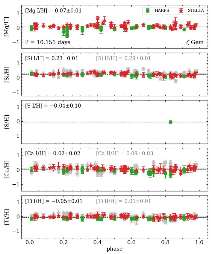
Figure B.5 shows the derived metallicities as a function of
the pulsation phase. Data plotted in this figure show that the
iron abundances are quite stable along the pulsation cycle. This
outcome applies to short-/long-period Cepheids and to Bump
Fig. 9. Atmospheric parameters derived by keeping fixed the effective Cepheids. We note that the current approach improves the results
temperature (previously obtained from the LDR method) in comparison obtained by Proxauf et al. (2018), since in their iron abundances
with the same parameters derived with T eff as a free parameter. The was still present a mild variation along the rising branch of large
panels show the comparison for the β Dor and ζ Gem stars. amplitude Cepheids (in our current results the dispersions are in
2
pyMOOGi: https://github.com/madamow/pymoogi
Article number, page 10 of 31R. da Silva et al.: A new and homogeneous metallicity scale for Galactic classical Cepheids
Fig. 10. Stellar metallicity measured for our sample of 20 calibrating Cepheids compared with results from literature. Top panel: metallicity as
a function of the Galactocentric distance from the current work (blue circles) and from literature (gray circles): Luck et al. (2011, LII); Luck &
Lambert (2011, LIII); Lemasle et al. (2013, LEM); Yong et al. (2006, YON). A linear regression (solid black line plus equation) fitted to the entire
sample is compared with the radial gradient provided by Ripepi et al. (2022) (dashed magenta line). The latter was artificially shifted to coincide
with the current radial gradient at RG = 10 kpc. The RG values are from Genovali et al. (2014). Bottom panel: same as the top, but as a function of
the logarithmic pulsation period. A linear regression (solid blue line plus equation) fitted to the current sample is also show.
most cases smaller than 0.05 dex). The improvement is mainly compared to another method normally used, in which the mini-
due to the very careful selection of the lines adopted to estimate mization process also includes T eff as a free parameter, we per-
the iron abundance. The difference is soundly supported by the formed a new and independent determination of the three atmo-
distribution of the standard deviations displayed in Fig. 7 for the spheric parameters plus abundances simultaneously for two vari-
Cepheids in common. The current standard deviations for both ables in our sample (β Dor and ζ Gem). The differences between
[Fe i/H] (violet) and [Fe ii/H] (green) lines (bottom panel) are our canonical approach and the literature approach are shown in
smaller by 30%-40% when compared with our previous inves- Fig. 9. The overall agreement is quite good over the entire tem-
tigation. Moreover and even more importantly, they also attain perature range. Indeed, the mean and the standard deviations at-
similar values. tain tiny values. The mean difference in effective temperature is
To further constrain the difference between the current and 55 K, and for the surface gravity it is 0.12 dex only, while the mi-
our previous investigation, Fig. 8 shows the comparison for both croturbulent velocities attain almost identical values. The quoted
the atmospheric parameters and the iron abundance. The agree- differences cause a small increase of 0.04 dex in the iron abun-
ment is remarkable over the entire temperature range. The mean dance when T eff is a free parameter. We note that we adopted the
and the standard deviations for the atmospheric parameters are same line list in the tests performed either with fixed or with free
well within the current uncertainties. The new iron abundances T eff .
are, on average, ∼0.1 dex more metal-poor. Owing to the sim- In closing this subsection, we also investigate whether the
ilarity in the atmospheric parameters, this difference seems an current iron abundances display any clear trend with the Galac-
obvious consequence of the new line list. tocentric distance (RG ). The top panel of Fig. 10 shows the iron
abundance as a function of RG for the calibrating Cepheids (blue
Several different approaches have been suggested in the lit- circles) and for Cepheids available in the literature (gray circles).
erature to estimate the atmospheric parameters of variable stars We performed a linear fit over the entire sample and we found
(Fukue et al. 2015; Jian et al. 2020; Lemasle et al. 2020; Mat- the following relation:
sunaga et al. 2021; Taniguchi et al. 2021; Romaniello et al.
2021). In the current investigation, the effective temperature is [Fe/H] = (−0.055 ± 0.003)RG + (0.43 ± 0.03) (2)
firstly derived using the LDR method, then the other atmospheric
parameters are estimated at fixed effective temperature. The ad- The current slope agrees quite well with similar estimates avail-
vantages of this approach have already been discussed in several able in the literature and, in particular, with the recent estimate
papers. To provide a more quantitative estimate of the differences of the iron radial gradient (dashed line) provided by Ripepi et al.
Article number, page 11 of 31A&A proofs: manuscript no. daSilvaetal2021
Fig. 11. [X/Fe] abundances as a function of metallicity (left panels) and of the logarithmic pulsation period (right panels) comparing our 20
calibrating Cepheids with stars from literature: LII: Luck et al. (2011); LIII: Luck & Lambert (2011); LEM: Lemasle et al. (2013); YON: Yong
et al. (2006). The error bars indicate our typical errors.
(2022). We note that, to overcome variations in the zero-point uncertainty is set to that typical value, namely: σ([Mg/H]) =
mainly introduced by innermost and outermost Cepheids, the 0.11, σ([Si i/H]) = 0.10, σ([Ca i/H]) = 0.18, σ([Ca ii/H]) = 0.18,
gradient from Ripepi et al. (2022) was artificially shifted to co- σ([Ti i/H]) = 0.14, and σ([Ti ii/H]) = 0.10 dex (for the sulfur
incide with the current radial gradient at RG = 10 kpc. abundances, the uncertainties come from the spectral synthesis).
The bottom panel of Fig. 10 shows the iron abundance as The estimate of these typical errors was done by calculating the
a function of the logarithmic pulsation period. Data plotted in median of the standard deviations listed in Table 8 for spectra
this panel agree quite well with similar estimates available in the having at least 2 lines of the same element/species.
literature. Moreover, they do not show any significant variation The adopted standard solar abundances for both iron and α
when moving from young (long-period) to less young (short- elements are from Asplund et al. (2009), namely: A(Fe) = 7.50,
period) classical Cepheids. A(Mg) = 7.60, A(Si) = 7.51, A(S) = 7.12, A(Ca) = 6.34,
and A(Ti) = 4.95, with A representing the typical logarithmic
notation where H is defined to be A(H) = 12.00. These values
6.2. α-element abundances
are in good agreement with the very recent determinations done
The abundances of the α elements were derived using pyMOOGi by Asplund et al. (2021), which were obtained using the most
as well (except sulfur, for which the abundances were estimated up-to-date atomic and molecular data.
using the spectral synthesis method - see Sect. 6.2.1). We used For both iron and α abundances, we evaluated the system-
the ab f ind driver, which requires as input i) the model atmo- atic differences for stars in common between the current inves-
spheres, calculated from the atmospheric parameters obtained tigation and measurements from literature: Luck et al. (2011),
for each star, and ii) a list of lines containing the wavelength, the Luck & Lambert (2011), Lemasle et al. (2013), and Yong et al.
atomic number, the lower-level excitation potential, the log g f , (2006) for iron and α elements, and Proxauf et al. (2018) for iron
and the measured equivalent widths. Table 8 lists the individ- only. The differences for all the investigated elements are listed
ual α-element abundances obtained for each spectrum together in Table 10. In order to perform a direct comparison, we applied
with the standard deviations and the number of lines used for these zero-point differences to the literature datasets by putting
each element. The mean abundances, weighted by the standard the iron and the α-element abundances in our metallicity scale.
deviations, and the corresponding standard errors are shown in The spectroscopic samples for which there are no variables in
Table 9. The same mean data are plotted in Figs. 11, 12, and B.6 common between our investigation and those available in the lit-
for our 20 calibrating Cepheids (blue circles) and for similar data erature, the homogenization of the abundances was performed in
available in the literature (gray circles). two steps. To be more specific, we have no variables in common
For cases in which the abundance of a given element at a with Yong et al. (2006), therefore, we first scaled their abun-
given phase is based on only one or two lines, or if the estimated dances to match those from Luck & Lambert (2011), and then
error is lower than a typical value for each element/species, the we scaled them to match our metallicity scale.
Article number, page 12 of 31You can also read


