A Distributed Quantum-Behaved Particle Swarm Optimization Using Opposition-Based Learning on Spark for Large-Scale Optimization Problem - MDPI
←
→
Page content transcription
If your browser does not render page correctly, please read the page content below
mathematics
Article
A Distributed Quantum-Behaved Particle Swarm
Optimization Using Opposition-Based Learning on
Spark for Large-Scale Optimization Problem
Zhaojuan Zhang 1 , Wanliang Wang 1, *                and Gaofeng Pan 2
 1   College of Computer Science and Technology, Zhejiang University of Technology, Hangzhou 310023, China;
     zjzhang@zjut.edu.cn
 2   Department of Computer Science and Engineering, University of South Carolina, Columbia, SC 29208, USA;
     gpan@email.sc.edu
 *   Correspondence: wwl@zjut.edu.cn

 Received: 30 September 2020; Accepted: 17 October 2020; Published: 23 October 2020

 Abstract: In the era of big data, the size and complexity of the data are increasing especially
 for those stored in remote locations, and whose difficulty is further increased by the ongoing
 rapid accumulation of data scale. Real-world optimization problems present new challenges to
 traditional intelligent optimization algorithms since the traditional serial optimization algorithm
 has a high computational cost or even cannot deal with it when faced with large-scale distributed
 data. Responding to these challenges, a distributed cooperative evolutionary algorithm framework
 using Spark (SDCEA) is first proposed. The SDCEA can be applied to address the challenge
 due to insufficient computing resources. Second, a distributed quantum-behaved particle swarm
 optimization algorithm (SDQPSO) based on the SDCEA is proposed, where the opposition-based
 learning scheme is incorporated to initialize the population, and a parallel search is conducted on
 distributed spaces. Finally, the performance of the proposed SDQPSO is tested. In comparison
 with SPSO, SCLPSO, and SALCPSO, SDQPSO can not only improve the search efficiency but also
 search for a better optimum with almost the same computational cost for the large-scale distributed
 optimization problem. In conclusion, the proposed SDQPSO based on the SDCEA framework has
 high scalability, which can be applied to solve the large-scale optimization problem.

 Keywords: large-scale optimization; spark; qpso; distributed computing; cooperative evolution;
 opposition-based learning

1. Introduction
      Nowadays, the development of the Internet of Things has promoted the accumulation of big
data. With the increasing complexity of real-world optimization problems, the traditional sequential
optimization algorithm may take a long time to complete a task and even cannot deal with it when
the data are stored in different places. For the large-scale optimization problem, the accumulation
of big data is overwhelming our capacity to analyze through classical techniques, and whose
difficulty is further increased by the ongoing rapid accumulation of data scale. This challenge is
even greater, especially for the large-scale optimization problem since many local best optimums make
the algorithm easily fall into a local optimum, or the computational cost becomes extremely high.
However, the traditional optimization algorithm even cannot deal with it when faced with large-scale
distributed data.

Mathematics 2020, 8, 1860; doi:10.3390/math8111860                       www.mdpi.com/journal/mathematics
Mathematics 2020, 8, 1860                                                                           2 of 21

      Responding to the challenge, distributed optimization is presented as an efficient strategy
to improve search efficiency and to reduce this complexity, which can overcome the deficiencies
of large-scale, high-dimensional, and complex features in real-world optimization problems.
Meanwhile, how to design an efficient distributed optimization algorithm to address such a challenge
has received considerable attention over the past decade. Consequently, a distributed framework has
become an effective strategy for the big data-driven optimization problem, since distributed computing
can improve the search efficiency of the evolutionary algorithm [1,2].
      Studies on distributed evolutionary algorithms based on the different distributed frameworks
have attracted considerable attention over recent years [3]. In 2004, Google [4] proposed a framework,
called MapReduce. As one of the most successful frameworks for distributed computing, it has been
widely adopted for analyzing massive, high-dimensional, and dynamic data. Up to date, particle
swarm optimization (PSO) plays an essential role in improving the quality of large-scale data, and how
to achieve it by distributing is a hot topic. McNabb et al. [5] first proposed a distributed PSO based
on MapReduce (MRPSO), which effectively decreases the computational cost. However, MRPSO is
not suitable for objectives that are easier to evaluate and is more significant for applications where the
computational cost is too expensive.
      The distributed optimization algorithm based on MapReduce can address the challenge for the
big data-driven optimization problem since the distributed algorithm is better than the non-distributed
algorithm concerning convergence speed. However, it takes a long time for MapReduce to deal with
computationally intensive operations such as iterative operations, which are especially noticeable
if the search space involves a large number of local best positions, or if the computational cost of
evaluation becomes very high. Therefore, MapReduce is not a good framework for tasks such as
evolutionary algorithms that involve more iterative operations. Conversely, Spark, a distributed
computing platform based on Memory, is more capable of iterative computing than MapReduce [6].
As a result, the distributed optimization algorithm based on Spark has attracted considerable attention
over the past few years.
      Although some studies have been achieved, the distributed optimization by using a distributed
framework still requires further research. Therefore, this paper proposes a distributed cooperative
evolutionary algorithm framework using Spark (SDCEA). The remainder of this paper is as follows.
Section 2 mainly presents the literature review, including real-world optimization applications,
large-scale optimization, distributed optimization using MapReduce, and distributed optimization
using Spark. Section 3 presents the main steps of the proposed SDCEA, the strategies of the distributed
and cooperative co-evolution based on SDCEA. Section 4 presents the methodology, including the
initialization and evolution process of the proposed SDQPSO. Section 5 presents the experiment on
five typical large-scale optimization test functions and has a discussion on the proposed SDCEA and
SDQPSO methodology for further research work. Finally, Section 6 presents the conclusions.

2. Literature Review

2.1. Real-World Optimization Applications
     To our knowledge, recent studies regarding real-world optimization problems remain a challenge
faced by current intelligent optimization algorithms.
     Ghasemi et al. [7] proposed an uncertain multi-objective model for earthquake evacuation
planning. In the proposed model, the total cost of the location-allocation and the amount of the
shortage of relief supplies are considered. Furthermore, the proposed model can be applied in a real
case study in Tehran in comparison with Non-Dominated Sorting Genetic Algorithm-II (NSGA-II)
and epsilon constraint method. The results indicate the superiority of the modified multiple-objective
particle swarm optimization (MMOPSO) over the other approaches.
Mathematics 2020, 8, 1860                                                                            3 of 21

     Later, Ghasemi et al. [8] discussed planning for pre-disaster multi-period location-allocation
inventory decisions. A robust simulation-optimization approach is presented to deal with the
uncertainty of demand for relief commodities first. Then, a customized genetic algorithm is proposed to
solve the resultant deterministic mathematical model. The results indicated that pre-disaster planning
can minimize time costs and ultimately reduce the relief time.
     For the green closed-loop supply chain under uncertainty problems, modifications of the
imperialist competitive algorithm (MICA) can obtain better solutions, which verified the efficiency and
performance of the proposed algorithm [9]. Goodarzian et al. [10] discussed how to obtain an optimal
solution for multi-objective pharmaceutical supply chain network (PSCN) problems. First, the PSCN
problem was formulated as a Mixed-Integer Non-Linear Programming model, and meta-heuristics
were selected to deal with uncertainty parameters. After a comparison of meta-heuristics for large-size
problems, the results indicated that multi-objective firefly algorithm (MOFFA) can find an acceptable
solution efficiently with a relatively low computational cost.
     Verdejo et al. [11] proposed a synchronization methodology based particle swarm optimization
to tune parameters of power system stabilizers (PSSs) in electric power systems (EPSs). The results
on different test systems indicate that it can improve the stability of the large-scale multi-machine
electric system.

2.2. Large-Scale Optimization
     To overcome the several shortcomings, e.g., premature convergence, low accuracy, and poor
global searching ability, Zhang et al. [12] proposed a novel simple particle swarm optimization
based on random weight and confidence term (SPSORC) for global optimization problems.
Later, Yildizdan et al. [13] proposed a hybrid bat algorithm and an artificial bee colony algorithm,
and inertia weight was incorporated into the bat algorithm. The result indicates that the hybrid
algorithm can produce successful and acceptable results. Furthermore, a new hybrid algorithm,
the annealing krill quantum particle swarm optimization (AKQPSO) algorithm, is proposed [14].
The optimized PSO by quantum behavior and optimized KH by simulated annealing show better
performance in both exploitation and exploration.

2.3. Distributed Optimization Using MapReduce
      Traditional optimization algorithms need to be modified to deal with increasing data sizes.
Jin (2008) et al. [15] first proposed an improved MapReduce by adding a hierarchical reduction stage
to MapReduce. This model is called MRPGA (MapReduce for parallel GAs), which can be adopted to
achieve a distributed genetic algorithm. Later, genetic algorithms and distributed algorithms based
on the MapReduce framework have been proposed one after another. Wu et al. [16] introduced the
divide and conquer strategy and simulated annealing algorithm into the ant colony algorithm (ACO).
MapReduce-based ACO was proposed by using a distributed environment of cloud computing,
which can improve the efficiency of the solution. Cheng et al. [17] parallelized the ant colony
optimization algorithm with dynamic positive and negative feedback based on the Haloop framework
built by the MapReduce.
      Xu et al. [18] proposed an improved cuckoo algorithm for the analysis of big data based
on MapReduce, which can search for a better optimum at a faster speed. Al-Madi et al. [19]
proposed a scalable design and implementation of a glowworm swarm optimization algorithm based
on MapReduce, which has a good clustering performance and achieves a very close to linear speedup.
Ding et al. [20] divided the whole population into N sub-populations and combined co-evolution and
MapReduce to share the results of all independent subsets based on cloud computing, which could
obtain a better adaptive balance between search and exploration of solutions.
      For the quantum optimization algorithm, Hossain et al. [21] proposed a parallel cluster particle swarm
optimization algorithm based on MapReduce by combining PSO and k-means algorithm, which can
deal with the problem for service decomposition in the mobile environment by using MapReduce.
Mathematics 2020, 8, 1860                                                                         4 of 21

Wang et al. [22] proposed a distributed co-evolutionary particle swarm optimization based on MapReduce,
which can shorten the search process of collaborative operation. Further, based on MapReduce,
Li et al. [23] and Ding et al. [24] studied the distributed quantum-behaved particle swarm optimization
by incorporating the local attractors and quantum rotating gates, and two different encoding and
decoding methods. Khalil et al. [25] proposed a MapReduce-based distributed whale algorithm
(MR-WOA) to improve the search efficiency for composition space. Furthermore, the speedup scales
linearly with increasing the number of computational nodes, which improves the scalability of WOA
for solving large-scale problems.

2.4. Distributed Optimization Using Spark
     For the large-scale global optimization problem, Cao et al. [26] proposed a parallel
cooperative particle swarm evolution algorithm combined with GPSO and LPSO by using Spark.
Dynamic grouping and multiple calculations are adopted to increase the degree of parallelism,
which makes sufficient exploration of the search space and speed up the convergence. Qi et al. [27]
proposed a two-stage parallel algorithm, including parallelization of fitness evaluation and
parallelization of genetic operations, the results show that the proposed algorithm outperforms
the sequential genetic algorithm in both test suite size and computational performance. Liu et al. [28]
proposed a parallel GA algorithm based on Spark, which is applied to design optimal deployment
schemes for sensor networks. Yuan et al. [29] proposed a Spark-based particle swarm optimization
algorithm with dynamic adaptive weight, which is adopted to optimize the input of the K-means
algorithm. The results show that the time spent in the execution process can be effectively reduced.
     Peng et al. [30] proposed a SparkCUDE algorithm where the Spark with a ring topology by
adaptively selecting crossover strategies and the CUDE algorithm is employed as the internal optimizer.
The results demonstrate the effectiveness and efficiency of the proposed approach for the large-scale
global optimization problem. Later, Teijeiro et al. [31] explored the differential evolution algorithm
under different population models, including the master–slave and the island-based DE schemes
by using Spark, which shows that the island model has the best performance and shows a decent
scalability. Sun et al. [32] proposed a distributed co-evolutionary algorithm for large scale flexible
scheduling problems, which divides the data based on sub-problems, and the results show that it has
better optimum and lower computational complexity.

3. A Distributed Cooperative Evolutionary Algorithm Framework Using Spark (SDCEA)

3.1. Background of the Distributed Framework
     In recent years, distributed frameworks have been widely used for machine learning, data mining,
image processing, and so on. Although the MapReduce is a simple batch computing model, which lacks
an effective mechanism for data sharing in various stages of parallel computing, it has been applied for
big data-driven optimization. For computationally intensive tasks, e.g., excessive iterative operations,
lower computation efficiency can be caused because of the frequently starting map and reduce
tasks. To overcome the shortcoming, Spark, a distributed computing framework based on Memory,
is proposed by the University of Berkeley. Indeed, Spark is an efficient framework to address the
challenge, whose difficulty lies in time consumption for iterative operations.
     When faced with big data-driven optimization problems, distributed computing frameworks
based on Spark have been proposed since Spark is efficient for evolutionary algorithms evolved through
iterative operations. Resilient distributed dataset (RDD) is adopted in Spark, and different operations
based on RDD are provided so that distributed data can be processed easily [33]. For dynamic
multi-objective optimization problems, Cordero et al. [34] proposed a software package using
Spark, called JMetal. Further, Duan et al. [35] proposed a Spark-based software framework for
parallel evolutionary algorithms (Spark-based PEAs), and three different particle swarm optimization
algorithms are implemented in parallel, which shows that the framework has a high search efficiency
Mathematics 2020, 8, 1860 5 of 21
for computationally expensive optimization problems. Furthermore, the above-mentioned Spark-based
software framework can make the algorithm in parallel easier, where JMetal is only proposed for
dynamic multi-objective optimization problems, and the Spark-based PEAs are mainly designed
concerning software Implementation. Generally speaking, distributed evolution is an effective way for
big data-driven optimization problems.
For the large-scale optimization problem, the algorithm may fall into a local optimum easily since
there are many local best optimums. Furthermore, the performance of the algorithm is determined
by different population distribution and data distribution strategies. Therefore, how to adopt the
distributed and parallel framework is a challenge faced by distributed optimization algorithms.
In this paper, a distributed cooperative evolutionary algorithm framework using Spark (SDCEA) is
proposed, which comprehensively considers computing distribution, population distribution, and data
distribution. The SDCEA can greatly improve the performance of computing efficiency while keeping
high fault tolerance and high scalability.
3.2. The Main Steps of the Proposed SDCEA Framework
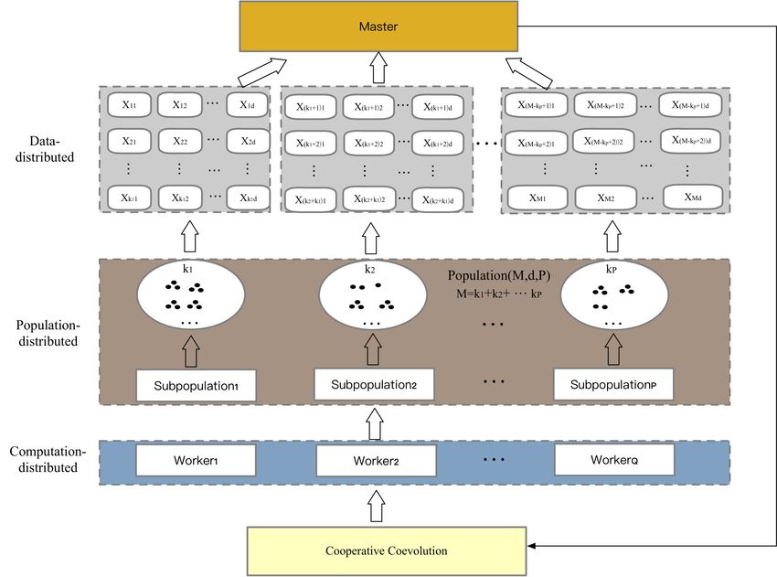
The SDCEA framework, as shown in Figure 1, mainly consists of three parts: distributed
computation, distributed population, and distributed data. The Spark distributed cluster environment
consists of a master node (Master) and multiple slave nodes (Workers), and the computing resource
corresponding to the whole workers is a resource pool. More importantly, the distributed computing
of the search is achieved by many distributed workers; thus, the computing resource pool is crucial to
the performance of algorithms.
Figure 1. The distributed cooperative evolutionary algorithm framework using Spark (SDCEA) framework.
The SDCEA framework is mainly designed for the evolutionary algorithm that adopts Spark as a
distributed computing platform. Furthermore, three distributed strategies are incorporated into the
SDCEA framework to address the challenge faced by big data-driven optimization problems. Based onMathematics 2020, 8, 1860 6 of 21
this framework, it can be found that the efficiency of distributed computing improved dynamically
with the increasing nodes of spark clusters. Therefore, it can be concluded that the SDCEA framework
is significant for large-scale optimization problems.
The main steps of the SDCEA framework are given as follows:
1. Configure a distributed computing cluster using Spark. Given Q workers and one master, where Q
workers are independent of each other. Based on the task mechanism, the distributed evolution is
divided into population distribution and data distribution. Furthermore, the master–slave model
is adopted for the proposed SDCEA framework.
2. Group the whole population into many sub-populations based on the parallelization, where each
sub-population consists of different individuals, and then each sub-population evolves
independently in parallel. Specifically, divide the whole population into P sub-populations
denoted by sub-population 1, sub-population 2, ..., and sub-population P, respectively.
3. The search space is partitioned into multiple subspaces for the whole population, and the
individual of each sub-population searches on the sub-spaces in parallel.
4. After each sub-population evolves separately for one iteration, the result is further collected
through the master. Specifically, the optimum on each search space found by the distributed
cooperation is collected by the master. Therefore, the global best optimum of the whole population
is achieved, and then the global best optimum is distributed to each worker. Finally, when each
worker receives it, the particle position and fitness evaluation of the population are updated.
The above steps 1–4 list a detailed procedure of the SDCEA framework, where each worker
searches in parallel first and then cooperate with the master. The master can collect the result of
all workers and further compute the global best position of the population at the current iteration.
The process is repeated until the search condition is reached, then the whole search process is finished.
3.3. Distributed and Cooperative Co-evolution Based on SDCEA
3.3.1. Population Distribution
Since distributed evolutionary strategies consist of two main types: population distribution,
where individuals of a sub-population are distributed to a different worker, and the same parameter
distribution of all sub-populations is adopted; data distribution, where the search space is partitioned
into blocks and then is computed in parallel. A distributed evolution model of master–slave cooperative
cooperation is proposed for the SDCEA framework, as shown in Figure 2. Furthermore, the population
is divided into several sub-populations, and then the distributed evolution of all sub-populations
is finished by several workers. Finally, search results are collected by the master among all
sub-populations. Consequently, the master obtains the best individual from the workers, and the
global best position is sent to all workers.
When populations are divided into several sub-populations, the population is partitioned in
parallel based on the degree of parallelism, and each sub-population is independent of each other.
Moreover, each subpopulation is evolved according to the update process of the evolutionary algorithm.
After one generation, the fitness is recomputed and the global best position of each subpopulation
is updated. From Figure 2, where Gbest P represents the global best position corresponding to
the P-th subpopulation and Gbest g represents the global best position of the whole population,
respectively. If the updated fitness of an individual is less than the previous fitness value of the
subpopulation, then the fitness value is updated as the global best position of the subpopulation.
Furthermore, the individual is selected as the current global best position of the subpopulation for the
current generation.Mathematics 2020, 8, 1860 7 of 21
Figure 2. The evolution model of master–slave cooperative cooperation.
3.3.2. Data Distribution
For the SDCEA framework, the whole search space is partitioned into several subspaces that
evolve independently towards the global best position. The data distribution is illustrated in Figure 3,
where the position of particles is parallelized as several subspaces. Furthermore, the performance of
the algorithm is much affected by the parallelism of partition. Assuming that the data are parallelized
into P groups, namely that the search space can be partitioned into P subspace, and thus the search
space is saved as P partitions. The search on each partition is performed serially but in parallel
between different partitions. Consequently, data have been parallelized based on the distributed
computing framework.
Figure 3. Data distribution of the proposed SDCEA framework.Mathematics 2020, 8, 1860 8 of 21
3.3.3. Distributed Cooperative Co-evolution
For the SDCEA framework, distributed search and cooperative cooperation of the population
is achieved based on the Spark. The cooperative co-evolution mainly includes two stages.
First, distributed co-evolution is performed independently by all individuals of each sub-population,
and each individual concerning all dimensions is updated. Second, further cooperation on the
candidate of the global best position is achieved between each worker and the master. Thus, the search
of the algorithm is finished through the distributed cooperation of the Spark cluster.
4. Methodology
4.1. SDQPSO Using Opposition-Based Learning
The QPSO is proposed by introducing quantum physics theory into the particle swarm
optimization algorithm, which significantly improves the global search ability of the particle.
However, there are still many shortcomings, such as premature phenomena and the diversity of
the population decreases through evolving. It is easy to fall into the local optimum if the search space
is composed of many local optimums, especially when the data are distributed or stored in different
places. To overcome the shortcomings of the QPSO algorithm, a distributed quantum-behaved particle
swarm optimization algorithm using spark based on the SDCEA framework is proposed (SDQPSO).
The initialization and update process of the SDQPSO algorithm is described below.
4.1.1. Population Initialization Using Opposition-Based Learning
The opposition-based learning (OBL) scheme has attracted considerable attention since it was
proposed in 2005 [36]. The main idea is to search in the opposite direction of a feasible solution,
and then to evaluate the original solution and opposite solution. Finally, find a better solution as the
individual for the next generation. The opposite point and opposite solution are defined below.
Definition 1. Opposite point. Let X = ( X1 , X2 , · · · , Xd ) be a point in a d-dimensional space, Xi ∈ [ ai , bi ],
where X1 , X2 , · · · , Xd are
real numbers, and i = 1, 2, · · · , d, respectively. Then the opposite point corresponding
to X is denoted by X e= X e1 , X
e2 , . . . , X
e d , and is given by
e i = a i + bi − X i
X (1)
Definition 2. Opposite learning. Given that X = ( X1 , X2 , · · · , Xd ) is a feasible solution of the algorithm and
Xe is its opposite solution. Let f ( x ) be the fitness evaluation function, and f ( Xe ) is its opposite fitness evaluation
function. Then the fitness value is evaluated at the initialization of the population. The learning continues with
Xe if the fitness value of f ( x ) is better than the fitness value of f ( X
e ), otherwise with X.
For the SDQPSO algorithm, the initialization of the population is achieved by adopting the
opposition-based learning scheme, which can improve the probability of the population to obtain a
better search space and further improve the search efficiency without prior knowledge.
4.1.2. Evolving through Generations
The evolution process of the SDQPSO is as follows: first, the master distributes the
sub-populations to different workers through the Spark cluster, or the data space has been distributed
to each worker; then the update process is performed independently and in parallel on workers.
The fitness of each particle is computed and then compared with the global best position on each
worker. Then, the personal best position denoted by Pbest is corresponds to each subpopulation,
where the personal best position of a particle is the best previous best position (i.e., the position with
the best fitness value). Furthermore, the global best position is defined as the best position amongMathematics 2020, 8, 1860 9 of 21
all the particles, which is denoted by Gbest g . The value of Gbest g is given by comparing through
each sub-population.
The mean best position (mbest) is defined as the mean position of the personal best positions in
the population. It is got by the master and sent to each worker, and it is given by
M M
Pbesti Pbest1 M Pbest2 M
Pbest M
mbest = ∑ M
=∑ ,∑
M i =1 M
,..., ∑
M
(2)
i =1 i =1 i =1
where M is the population size, Pbesti represents the personal best position of the i-th
particle, respectively.
Since the evolution process only considers individual best position and global cooperation,
the global best position of each sub-population is considered during the improved evolution process.
This can fully reflect the first-stage cooperation among individuals in each sub-population. For each
worker, the local attractor is given by
(1 − µ ) (1 − µ )
Pid = µPbest + Gbest j + Gbest g (3)
2 2
where Pid represents the local attractor of the i-th individual, µ is a random number uniformly
distributed on (0, 1), and d is the particle dimension, respectively. Moreover, Gbest j represents the
global best position of the j-th subpopulation, and Gbest g represents the global best position of the
whole population.
Further, on each worker, the position of each particle in the sub-population is updated generation
by generation during the evolution process, and it is given by
Pid (t) + β |mbest(t) − Xid (t)| × ln 1 , if u < 0.5
Xid (t + 1) = u (4)
Pid (t) − β |mbest(t) − Xid (t)| × ln 1 , if u ≥ 0.5
u
where Xid (t + 1) is the current position of the particle in the t + 1 generation, and u is a random number
uniformly distributed on (0, 1), respectively. Furthermore, β is a contraction–expansion coefficient
from 0.5 to 1.0, which is used to control the convergence speed of the particles. Different β can affect
the convergence speed of the algorithm. Generally, the value of β is taken as
(1.0 − 0.5) × ( MAXITER − t)
β= + 0.5 (5)
MAXITER
where MAXITER is the maximum iteration and t represents the current iteration.
Finally, the global best position of each sub-population searched in parallel is collected
by the master and the master analysis whether the termination condition is reached. If the
termination condition is reached, then the global best position of the whole population is got.
Otherwise, the updated parameters, Gbest g and mbest are distributed to each worker. The whole
evolution is repeated until the termination condition is reached, and then the distributed search of the
search space based on the SDCEA framework is completed.
4.2. Evolution Process of the Proposed SDQPSO
The evolution process of the whole SDQPSO algorithm is shown in Figure 4, where Fes represents
the function evaluations, and Maxevals represents the maximum function evaluations, respectively.
The search space saved as RDDs is partitioned into several subspaces, and each sub-population
searches in parallel on each worker. The master collects the results of all workers first and then
distributes them to the worker. Through the cooperation of the master and each worker, the whole
distributed search process is finished when the termination condition is reached.Mathematics 2020, 8, 1860 10 of 21
Figure 4. The evolution process of the distributed quantum-behaved particle swarm optimization
(SDQPSO) algorithm.
The main steps of the SDQPSO algorithm are as follows:
1. The population is initialized by adopting opposition-based learning scheme on the master, where
the population size is M, the current position is X = ( X1 , X2 , · · · , Xd ), the personal best position
is Pbest, and the global best position is Gbest g . Furthermore, the positions of the population are
within the range of [ Xmin , Xmax ].
2. According to Equation (2), the mean best position denoted by mbest is updated by averaging the
personal best position on the master.
3. The population is divided into P sub-populations on the master, then the sub-population and
mbest are distributed to each worker. Moreover, the computing resource is distributed to each
subpopulation, and the search space is partitioned into several search subspaces.
4. According to Equation (3), the local attractor of the particle denoted by Pid is updated on the
worker, where i = 1, 2, . . . M.
5. Each subpopulation on the worker evolves independently generation by generation, and the
position of each particle is updated according to the Equation (4).
6. The fitness value of each particle is evaluated on the worker. When compared with Pbest, if the
current fitness value is better than the previous personal best position, then Pbest is updated,
otherwise not.Mathematics 2020, 8, 1860 11 of 21
7. For each worker, the particle with the best fitness value of each subpopulation is set as Gbest j .
8. The updated Gbest j of each subpopulation and the current position are sent to the master.
9. The Gbest j of all the sub-populations on the worker is sent to the master, where j = 1, 2, . . . P.
Furthermore, each Gbest j is compared with Gbest g , if it is less than Gbest g , the global best position
is updated, otherwise not. Then the updated Gbest g is distributed to each worker.
Repeat Step 2–Step 9. The evolution process is finished if the termination condition is reached,
and finally the global best position denoted by Gbest g and the personal best position denoted by Pbest
are achieved; if the termination condition is not reached, go to Step 2.
5. Results and Discussion
5.1. Experimental Environment and Parameter Settings
5.1.1. Experimental Environment
The experimental environment of the Spark cluster is configured as follows: Dell PowerEdge R930
with Xeon(R) CPU E7-4820V4 @ 2.0 GHz *20, 256 GB memory and 6 TB hard disk. The configuration
of the Spark platform is described in Table 1, where the distributed cluster environment is virtualized
with VMware, and the Spark cluster consists of four nodes.
Table 1. Spark cluster for distributed computing.
Spark Cluster Platform Configuration
Distributed computing nodes 1 Master and 3 Workers
System VMware ESXi 6.5.0, Ubuntu 16.04
Framework version Hadoop 3.2.1, Spark 2.4.5
Software version Scala 2.11.12, java 1.8.0, Sbt 1.1.6
5.1.2. Test Problems and Parameter Settings
For the large-scale optimization problem, two typical test functions with different time complexity
were selected to verify the performance of SDQPSO. As shown in Table 2, the test functions represent
five different types of optimization problems, and the time complexity of test functions is linear or
quadratic. Furthermore, four test functions were selected with linear time complexity for low-cost
optimization problems: Sphere, Rosenbrock, Rastrigin, Griewank; a test function with quadratic
time complexity was selected for high-cost optimization problems: Schwefel 1.2. In addition,
each experiment was run 30 times independently.
Table 2. Test functions.
Test Function Name
= ∑in=1 xi2
hF1 ( x ) Sphere
2 i
F2 ( x ) = ∑in=−11 100 xi+1 − xi2 + ( x i − 1)2 Rosenbrock
F3 ( x ) = ∑in=1 xi2 − 10 cos (2πxi ) + 10
Rastrigin
√
F4 ( x ) = 1/4000 ∑in=1 xi2 − ∏in=1 cos xi / i + 1 Griewank
2
F5 ( x ) = ∑in=1 ∑ij=1 x j Schwefel 1.2
SDQPSO is compared with three different existing distributed particle swarm optimizers; namely,
Spark-based distributed particle swarm optimizer (SPSO) [37], Spark-based comprehensive learning
particle swarm optimizer (SCLPSO) [38], and Spark-based aging leader and challengers particle swarm
optimizer (SALCPSO) [39]. All the experimental parameters of the compared algorithms are set the
same as the original paper. The population size is set to 100, and β is set to 0.5 in SDQPSO. In thisMathematics 2020, 8, 1860 12 of 21
paper, the performance of the SDQPSO algorithm based on the SDCEA framework is tested from three
different perspectives: test functions with different time complexity, different dimensions, and different
function evaluations, respectively. Based on 30 independent runs, optimization performance and
computational cost are analyzed. For computational cost, the mean running time and function
evaluation time are reported.
5.2. Comparison with SDQPSO, SPSO, SCLPSO, and SALCPSO
5.2.1. Optimization Performance on Four Low-Cost Test Functions
To evaluate the optimization performance of SDQPSO, SDQPSO is compared with SPSO, SCLPSO,
and SALCPSO. Since Spark is a distributed framework that is efficient for the large-scale optimization
problem, the test function is designed with a higher dimension and more expensive computational
cost. The dimension is set to 100,000, and the function evaluations are set to 5000. For F1, F2,
F3, and F4, the results obtained by SDQPSO, SPSO, SCLPSO, and SALCPSO are shown in Table 3.
Furthermore, Wilcoxon’s rank sum test is used to represent Robust Statistical Tests to demonstrate the
performance of the proposed SDQPSO. The significance level is set to 0.05. “+” means the compared
algorithm performs significantly better than the proposed SDQPSO; “-” means the compared algorithm
performs statistically worse than the proposed SDQPSO; “=” refers to non-comparable between the
compared algorithm and the proposed SDQPSO.
In this paper, mean value, maximum value (max value), minimum value (min value), and standard
variance are listed to evaluate the optimization performance, and the better-obtained values are
indicated with bold fonts. As shown in Table 3, it can be found that the proposed SDQPSO has
achieved better optimums on F2 in terms of the mean value, max value, min value, and standard
variance. Furthermore, SALCPSO has achieved a better standard variance on F1, F3, and F4, whereas
SDQPSO is better for mean value, max value, and min value. In addition, the optimization performance
of the four compared algorithms has a relatively smaller difference on F3. In comparison with SPSO,
SCLPSO, and SALCPSO, SDQPSO can achieve relatively competitive performance on F1, F2, and F4.
According to the statistical results of 30 times on the functions, it can be concluded that the optimization
performance of SDQPSO is the comprehensively best on all values, and SPSO is the second-best.
Table 3. Optimization performance on four functions.
Function SDQPSO SPSO SCLPSO SALCPSO
Min 2.74 × 10⁵ 1.59 × 10⁶ 1.75 × 10⁶ 2.69 × 10⁶
Mean 2.86 × 10⁵ 1.61 × 10⁶ (-) 1.75 × 10⁶ (-) 2.70 × 10⁶ (-)
F1
Max 2.97 × 105 1.62 × 10⁶ 1.76 × 10⁶ 2.70 × 10⁶
Std 7.41 × 10³ 9.97 × 10³ 6.63 × 10³ 4.33 × 10³
Min 1.31 × 10⁹ 7.28 × 10⁹ 7.35 × 10⁹ 1.69 × 10¹⁰
Mean 1.32 × 10⁹ 7.38 × 10⁹ (-) 7.44 × 10⁹ (-) 1.69 × 10¹⁰ (-)
F2
Max 1.32 × 109 7.49 × 10⁹ 7.53 × 10⁹ 1.70 × 10¹⁰
Std 3.44 × 10⁶ 6.74 × 10⁷ 5.30 × 10⁷ 3.26 × 10⁷
Min 1.27 × 10⁶ 2.55 × 10⁶ 2.73 × 10⁶ 3.61 × 10⁶
Mean 1.28 × 10⁶ 2.59 × 10⁶ (-) 2.74 × 10⁶ (-) 3.61 × 10⁶ (-)
F3
Max 1.29 × 106 2.60 × 10⁶ 2.76 × 10⁶ 3.62 × 10⁶
Std 7.03 × 10³ 1.55 × 10⁴ 7.81 × 10³ 3.37 × 10³
Min 6.73 × 101 3.97 × 10² 4.36 × 10² 6.73 × 10²
Mean 7.16 × 101 4.03 × 10² (-) 4.37 × 10² (-) 6.75 × 10² (-)
F4
Max 7.34 × 101 4.10 × 10² 4.40 × 10² 6.76 × 10²
Std 1.93 × 100 3.43 × 100 1.38 × 100 8.46 × 10⁻¹
+/=/- 0/0/4 0/0/4 0/0/4Mathematics 2020, 8, 1860 13 of 21
5.2.2. Optimization Performance under Different Function Dimensions
To test the performance of the SDQPSO under different function dimensions, the Schwefel
1.2 function with quadratic time complexity is selected since it can highlight the advantage of the
distributed computing using Spark. For Schwefel 1.2, the dimension is set to 10, 100, 1000, 10,000,
100,000. Furthermore, based on our experience, the computational cost of the Schwefel 1.2 function is
very high for large-scale optimization problems, so the function evaluation is set to 500. In addition,
since the optimization performance of the distributed optimizer under different dimensions is a crucial
issue, the comparison of different function evaluations is specifically described in Section 5.2.3 when
the function dimension is set to 100,000.
The optimization performance of SDQPSO, SPSO, SCLPSO, and SALCPSO under different
function dimensions is shown in Table 4. It can be seen from Table 4 that SDQPSO has achieved
better optimums on the mean value, max value, min value, and standard variance, except that
SPSO has achieved the best standard variance when the dimension is 100,000. From Table 4, it is
clear that the optimum obtained by SDQPSO is much closer to the optimum in theory when the
dimension is 10. In addition, the difficulty of obtaining the optimal solution increases gradually with
the dimension increasing. Furthermore, the performance of SCLPSO is relatively worse than the other
three algorithms, but SDQPSO, SPSO, SCLPSO, and SALCPSO can achieve a relatively close optimum.
Comprehensively, on the four values, SPSO is the second-best, and then SALCPSO, and the proposed
SDQPSO adopting the opposition-based learning scheme has a competitive optimization performance.
Table 4. Optimization performance under different function dimensions.
Dimension SDQPSO SPSO SCLPSO SALCPSO
Min 1.22 ×100 7.19 × 100 3.29 × 101 2.19 × 101
Mean 6.94 × 100 1.81 × 101 (-) 9.93 × 101 (-) 4.43 × 101 (-)
10
Max 1.99 × 101 2.69 × 101 1.60 × 10² 9.17 × 101
Std 4.97 × 100 5.58 × 100 2.98 × 101 1.56 × 101
Min 1.21 × 10³ 1.79 × 10³ 6.41 × 10³ 3.47 × 10³
Mean 2.00 × 10³ 2.96 × 10³ (-) 9.00 × 10³ (-) 5.64 × 10³ (-)
100
Max 2.60 × 103 4.20 × 10³ 1.21 × 10⁴ 1.01 × 10⁴
Std 4.35 × 10² 5.63 × 10² 1.46 × 10³ 1.32 × 10³
Min 1.47 × 10⁵ 1.51 × 10⁵ 5.23 × 10⁵ 2.79 × 10⁵
Mean 2.34 × 10⁵ 2.85 × 10⁵ (-) 8.73 × 10⁵ (-) 5.24 × 10⁵ (-)
1000
Max 2.94 × 105 3.94 × 10⁵ 1.25 × 10⁶ 8.39 × 10⁵
Std 4.15 × 10⁴ 5.28 × 10⁴ 1.95 × 10⁵ 1.17 × 10⁵
Min 1.50 × 10⁷ 1.89 × 10⁷ 5.44 × 10⁷ 3.85 × 10⁷
Mean 2.53 × 10⁷ 2.98 × 10⁷ (-) 8.98 × 10⁷ (-) 5.44 × 10⁷ (-)
10,000
Max 3.56 × 107 4.68 × 10⁷ 1.53 × 10⁸ 7.93 × 10⁷
Std 5.68 × 10⁶ 6.23 × 10⁶ 1.95 × 10⁷ 1.01 × 10⁷
Min 1.75 × 10⁹ 2.26 × 10⁹ 4.44 × 10⁹ 3.25 × 10⁹
Mean 2.59 × 10⁹ 3.16 × 10⁹ (-) 8.89 × 10⁹ (-) 5.47 × 10⁹ (-)
100,000
Max 3.42 × 109 4.18 × 10⁹ 1.35 × 10¹⁰ 9.05 × 10⁹
Std 7.16 × 10⁸ 5.26 × 10⁸ 2.11 × 10⁹ 1.32 × 10⁹
+/=/- 0/0/5 0/0/5 0/0/5
5.2.3. Optimization Performance under Different Function Evaluations
For the large-scale optimization problem, the optimization performance of SDQPSO under
different function evaluations is discussed. A high-cost Schwefel 1.2 function is selected. Moreover,
five function evaluations are set to 1000, 2000, 3000, 4000, 5000, and the dimension is set to 100,000.
The optimization performance of SDQPSO, SPSO, SCLPSO, and SALCPSO under different
function evaluations are shown in Table 5. From Table 5, it can be found that SDQPSO and SPSOMathematics 2020, 8, 1860 14 of 21
have better optimums. When the function evaluation is set to 1000, SDQPSO could obtain the best
optimum on min value, max value, and standard variance, but is worse than SPSO on the mean
value. When the function evaluations are 2000 and 4000, SDQPSO could achieve a better standard
variance but with a slightly inferior performance than SPSO on the optimum. Furthermore, when the
function evaluations are 3000 and 5000, SDQPSO is very close to SPSO on the four values: mean value,
max value, min value, and standard variance. The optimum obtained by SDQPSO has a superior
performance when compared with SCLPSO and SALCPSO. In conclusion, SDQPSO could obtain a
competitive performance for the large-scale and high-cost optimization problem.
Table 5. Optimization performance under different function evaluations.
Evaluation SDQPSO SPSO SCLPSO SALCPSO
Min 1.43 × 10⁹ 1.49 × 10⁹ 4.20 × 10⁹ 2.61 × 10⁹
Mean 2.54 × 10⁹ 2.21 × 10⁹ (=) 7.96 × 10⁹ (-) 4.20 × 10⁹ (-)
1000
Max 2.99 × 109 3.06 × 10⁹ 1.08 × 10¹⁰ 5.76 × 10⁹
Std 4.10 × 10⁸ 4.48 × 10⁸ 1.59 × 10⁹ 6.80 × 10⁸
Min 1.42 × 10⁹ 1.07 × 10⁹ 3.67 × 10⁹ 2.21 × 10⁹
Mean 2.31 × 10⁹ 1.78 × 10⁹ (+) 6.82 × 10⁹ (-) 3.33 × 10⁹ (-)
2000
Max 2.87 × 109 2.50 × 10⁹ 9.90 × 10⁹ 4.52 × 10⁹
Std 3.21 × 10⁸ 3.40 × 10⁸ 1.50 × 10⁹ 6.74 × 10⁸
Min 1.61 × 10⁹ 1.13 × 10⁹ 3.76 × 10⁹ 2.17 × 10⁹
Mean 2.32 × 10⁹ 1.64 × 10⁹ (+) 5.59 × 10⁹ (-) 3.20 × 10⁹ (-)
3000
Max 2.75 × 109 2.54 × 10⁹ 8.09 × 10⁹ 3.92 × 10⁹
Std 4.12 × 10⁸ 3.01 × 10⁸ 1.05 × 10⁹ 4.58 × 10⁸
Min 1.88 × 10⁹ 1.10 × 10⁹ 3.57 × 10⁹ 2.20 × 10⁹
Mean 2.16 × 10⁹ 1.51 × 10⁹ (+) 5.67 × 10⁹ (-) 2.89 × 10⁹ (-)
4000
Max 2.44 × 109 2.02 × 10⁹ 7.52 × 10⁹ 4.08 × 10⁹
Std 1.85 × 10⁸ 2.04 × 10⁸ 9.85 × 10⁸ 4.50 × 10⁸
Min 1.63 × 10⁹ 1.16 × 10⁹ 4.11 × 10⁹ 2.02 × 10⁹
Mean 2.11 × 10⁹ 1.53 × 10⁹ (+) 5.52 × 10⁹ (-) 2.68 × 10⁹ (-)
5000
Max 2.85 × 109 1.96 × 10⁹ 7.50 × 10⁹ 4.01 × 10⁹
Std 3.80 × 10⁸ 1.93 × 10⁸ 8.23 × 10⁸ 4.14 × 10⁸
+/=/- 4/1/0 0/0/5 0/0/5
5.3. Performance on the Running Time and Function Evaluation Proportion
5.3.1. Running Time and Function Evaluation Proportion on Four Low-Cost Test Functions
For the time metrics, the running time and function evaluation time were reported. The function
dimension is set to 100,000, and the function evaluation is set to 5000. The time performance of SDQPSO,
SPSO, SCLPSO, and SALCPSO on four different functions is shown in Figure 5, where Figure 5a–d
represent the time metrics of Sphere, Rosenbrock, Rastrigin, and Griewank, respectively. For Figure 5,
different colored histograms represent different time metrics, blue for the running time, and orange for
the function evaluation time.
For the running time, it can be found that SCLPSO has the highest computational cost on the four
low-cost test functions with linear time complexity, followed by SDQPSO. Furthermore, SPSO and
SALCPSO could obtain lower computational cost, and the running time of the two algorithms are very
close. Furthermore, the function evaluation time of SDQPSO, SPSO, SCLPSO, and SALCPSO is very
close, and the function evaluation proportion is small which means that the function evaluation only
takes less time. Generally speaking, compared with SPSO, SCLPSO, and SALCPSO, SDQPSO can keep
a relatively competitive performance on the time metric.Mathematics 2020, 8, 1860 15 of 21
Figure 5. The time metrics on Sphere, Rosenbrock, Rastrigin, Griewank. (a) Time on Sphere, (b) time
on Rosenbrock, (c) time on Rastrigin, (d) time on Griewank.
The function evaluation proportion represents the proportion between the function evaluation
time and the running time. The function evaluation proportion of Sphere, Rosenbrock, Rastrigin,
and Griewank is shown in Figure 6, where four different colors represent the evaluation proportion of
different functions, respectively. From Figure 6, it can be found that the function evaluation proportion
of SCLPSO is the best, followed by SDQPSO, SPSO, and SALCPSO. However, the result shows that
the function evaluation is less time-consuming on the four low-cost test functions, ranging from 7.5%
to 15%. In summary, the experimental results verified the time complexity of the four low-cost test
functions. Furthermore, the SDQPSO using the opposition-based learning scheme could obtain better
function evaluation proportion when faced with the low-cost optimization problem.
Figure 6. The fun evaluation proportion on Sphere, Rosenbrock, Rastrigin, and Griewank.Mathematics 2020, 8, 1860 16 of 21
5.3.2. Running Time and Function Evaluation Proportion under Different Dimensions
For the large-scale optimization problem, a high-cost Schwefel 1.2 function with quadratic time
complexity is tested. The dimensions are set to 10, 100, 1000, 10,000, 100,000. The mean running times
of SDQPSO, SPSO, SCLPSO, and SALCPSO under different dimensions are shown in Figure 7, it is
clear that the mean running time of the four algorithms is very close. When the dimension is less than
1000, the mean running time of SDQPSO and SPSO, SCLPSO, and SALCPSO is less than 1 second,
and when the dimension is 10,000, the mean running time increases to nearly 10 seconds. In addition,
the mean running time increases drastically to more than 100 seconds when the dimension is set
to 100,000.
Figure 7. The running time under different dimensions.
The function evaluation proportion of SDQPSO, SPSO, SCLPSO, and SALCPSO under different
dimensions are shown in Figure 8. Since the computational cost of the algorithm is low, which results
in the function evaluation proportion being relatively high when dimensions are set to 10 and 100.
When the dimension is 1000, the function evaluation proportion of all algorithms is lower than that of
other dimensions, dimension and the function evaluation proportion of the four algorithms increases
with the further increase of dimensions. Furthermore, SCLPSO has the largest function evaluation
proportion among all algorithms, reaching nearly 75% when the dimension is 1000, and SDQPSO
outperforms SCLPSO.
Figure 8. The function evaluation proportion under different dimensions.Mathematics 2020, 8, 1860 17 of 21
5.3.3. Running Time and Function Evaluation Proportion under Different Function Evaluations
To verify the performance of SDQPSO under different function evaluations, the function
evaluations are set to 1000, 2000, 3000, 4000, 5000, respectively. In addition, the dimension is set
to 100,000, and the high-cost Schwefel 1.2 function is selected for the test. The mean running time of
SDQPSO, SPSO, SCLPSO, and SALCPSO under different function evaluations is shown in Figure 9.
From Figure 9, it can be found that the running time of the four algorithms increases linearly with
the function evaluation increasing. Furthermore, the running time of SDQPSO, SPSO, SCLPSO,
and SALCPSO is in an order of magnitude, and is very close to each other.
The function evaluation proportion under different function evaluations is illustrated in Figure 10.
In comparison with SPSO, SALCPSO, and SDQPSO, the decline of function evaluation proportion of
SCLPSO is the relatively best with the function evaluations increasing. Furthermore, for the function
evaluation proportion, the proposed SDQPSO has achieved the second-best while SCLPSO is the
best among all algorithms when the dimension ranges from 2000 to 5000. Further analysis is given
in Figure 10, it can be seen that the SDQPSO, SPSO, SCLPSO, and SALCPSO have a higher function
evaluation proportion for the large-scale and high-cost optimization problem. Generally speaking,
the experimental result verified the characteristics of the Schwefel 1.2 function, which means that the
computational cost of the function with quadratic time complexity is high.
Figure 9. The running time under different function evaluations.
Figure 10. The function evaluation proportion under different function evaluations.Mathematics 2020, 8, 1860 18 of 21
5.4. Discussion
With the ongoing rapid accumulation of data scale, and the increasing complexity of real-world
optimization problems, new challenges faced by traditional intelligent optimization algorithms are
increasing. To deal with the massive, high-dimensional, and dynamic challenge faced by the large-scale
optimization problem, a distributed cooperative evolutionary algorithm framework using Spark is
proposed first. Furthermore, the proposed framework can be extended with the increasing computing
resources, e.g., it can be extended to 10 nodes, 100 nodes. It means that the SDCEA is very flexible and
has good scalability regardless of the node size.
More importantly, the distributed optimization algorithm based on the SDCEA can be applied
to address the challenge in the other similar optimization problems. That is, the crucial issue is
how to implement an algorithm in a distributed way, so further study is deserved focusing on
the distributed optimization framework. When faced with the problem of lower computational
efficiency and higher computational cost caused by big data, the SDCEA proposed in this paper
and the distributed optimization algorithms can be applied to solve the above-mentioned challenges.
Therefore, how to design the distributed and cooperative co-evolution from the serial algorithm to the
big data-driven optimization is significant for real-world optimization problems.
Through further analysis of the results, it can be found that for the large-scale and low-cost
optimization problem, the performance on time metrics of the SDCEA is not competitive since
communication takes a long time through distributed computing. This means that distributed
computing is an effective strategy when faced with big data, and the larger the data are, the greater
the advantage will be. The running time of the algorithm mainly depends on the parallelism of the
algorithm, and the computational cost of each subpopulation directly affects the convergence speed
of the whole population. Too much parallelism means that there are too many tasks, which can
increase the overall computational cost. Furthermore, too few partitions can lead to unreasonable
use of computing resources, which increases the memory requirements for each worker, and if the
partition is not reasonable, which can result in data skew problems. Therefore, how to divide data in
parallel according to computing resources and search space is of great significance.
The communication of the master–slave distribution model is very time-consuming and inefficient;
thus, how to carry out the cooperation to reduce the communication time among the individuals of each
subpopulation is worthy of further discussion. Furthermore, how to design and implement a novel and
efficient framework based on big data platforms, e.g., MapReduce and Spark, to meet the increasing
requirements when faced with big data is still significant for large-scale optimization problems.
6. Conclusions
In order to address the challenge faced by the big data-driven optimization problem,
this paper first provides a literature review of the distributed intelligent optimization algorithms.
Second, a distributed cooperative evolutionary algorithm framework using Spark is proposed,
which combines distributed computing, population distribution, data distribution, and distributed
co-evolution. Third, the SDQPSO by adopting the opposition-based learning scheme to initialize
and be implemented in parallel based on the SDCEA framework. Finally, the performance of
the SDQPSO under different functions, different dimensions, and different fitness evaluations are
discussed, and three distributed optimizers, namely, SPSO, SCLPSO, and SALCPSO are selected
to compare.
For the large-scale optimization problem, the proposed SDQPSO can obtain relatively better
optimum values on low-cost functions. Moreover, for the high-cost and large-scale optimization
problem, it could obtain a relatively competitive performance on function evaluation proportion
and computational cost. Furthermore, the results show that the opposition-based learning scheme
improves the probability of the population to obtain a better search space without prior knowledge.
In conclusion, the proposed SDCEA framework can improve search efficiency by using Spark, and it
has high scalability that can be applied to address the complexity of large-scale optimization problems.Mathematics 2020, 8, 1860 19 of 21
Author Contributions: Conceptualization, Z.Z.; methodology, W.W.; validation, G.P.; formal analysis, Z.Z.
and G.P.; investigation, Z.Z.; resources, Z.Z.; data curation, G.P.; writing—original draft preparation, Z.Z.;
writing—review and editing, W.W.; visualization, G.P.; supervision, W.W.; project administration, W.W.; funding
acquisition, W.W. All authors have read and agreed to the published version of the manuscript.
Funding: This work was funded by the National Natural Science Foundation of China grant numbers 61873240.
The funding body did not play any role in the design of the study and collection, analysis, and interpretation of
data and writing the manuscript.
Acknowledgments: The authors wish to thank the editors and anonymous reviewers for their valuable comments
and helpful suggestions which greatly improved the paper’s quality. We would like to thank Marilyn E. Gartley
for excellent and professional copy-editing of the paper. This work was cooperated with the Department of
Computer Science and Engineering at University of South Carolina.
Conflicts of Interest: The authors declare no conflict of interest.
References
1. Gong, Y.J.; Chen, W.N.; Zhan, Z.H.; Zhang, J.; Li, Y.; Zhang, Q.; Li, J.J. Distributed evolutionary algorithms
and their models: A survey of the state-of-the-art. Appl. Soft Comput. 2015, 34, 286–300. [CrossRef]
2. Wang, W.L. Artificial Intelligence: Principles and Applications; Higher Education Press: BeiJing, China, 2020.
3. Wang, W.L.; Zhang, Z.J.; Gao, N.; Zhao, Y.W. Research progress of big data analytics methods based on
artificial intelligence technology. Comput. Integr. Manuf. Syst. 2019, 25, 529–547.
4. Dean, J.; Ghemawat, S. MapReduce: Simplified Data Processing on Large Clusters. Commun. ACM 2008, 51,
107–113.
5. McNabb, A.W.; Monson, C.K.; Seppi, K.D. Parallel pso using mapreduce. In Proceedings of the 2007 IEEE
Congress on Evolutionary Computation, Singapore, 25–28 September 2007; pp. 7–14.
6. Zaharia, M.; Chowdhury, M.; Franklin, M.J.; Shenker, S.; Stoica, I. Spark: Cluster computing with working
sets. HotCloud 2010, 10, 95.
7. Ghasemi, P.; Khalili-Damghani, K.; Hafezalkotob, A.; Raissi, S. Uncertain multi-objective multi-commodity
multi-period multi-vehicle location-allocation model for earthquake evacuation planning. Appl. Math. Comput.
2019, 350, 105–132. [CrossRef]
8. Ghasemi, P.; Khalili-Damghani, K. A robust simulation-optimization approach for pre-disaster multi-period
location–allocation–inventory planning. Math. Comput. Simul. 2020, 179, 69–95. [CrossRef]
9. Fakhrzad, M.B.; Goodarzian, F. A fuzzy multi-objective programming approach to develop a green
closed-loop supply chain network design problem under uncertainty: Modifications of imperialist
competitive algorithm. RAIRO-Oper. Res. 2019, 53, 963–990. [CrossRef]
10. Goodarzian, F.; Hosseini-Nasab, H.; Muñuzuri, J.; Fakhrzad, M.B. A multi-objective pharmaceutical supply
chain network based on a robust fuzzy model: A comparison of meta-heuristics. Appl. Soft Comput. 2020,
92, 106331. [CrossRef]
11. Verdejo, H.; Pino, V.; Kliemann, W.; Becker, C.; Delpiano, J. Implementation of Particle Swarm Optimization
(PSO) Algorithm for Tuning of Power System Stabilizers in Multimachine Electric Power Systems. Energies
2020, 13, 2093. [CrossRef]
12. Zhang, X.; Zou, D.; Shen, X. A novel simple particle swarm optimization algorithm for global optimization.
Mathematics 2018, 6, 287. [CrossRef]
13. Yildizdan, G.; Baykan, O.K. A new hybrid BA-ABC algorithm for global optimization problems. Mathematics
2020, 8, 1749. [CrossRef]
14. Wei, C.L.; Wang, G.G. Hybrid Annealing Krill Herd and Quantum-Behaved Particle Swarm Optimization.
Mathematics 2020, 8, 1403. [CrossRef]
15. Jin, C.; Vecchiola, C.; Buyya, R. MRPGA: An extension of MapReduce for parallelizing genetic algorithms.
In Proceedings of the 2008 IEEE Fourth International Conference on eScience, Indianapolis, IN, USA,
7–12 December 2008; pp. 214–221.
16. Wu, H.; Ni, Z.W.; Wang, H.Y. MapReduce-based ant colony optimization. Comput. Integr. Manuf. Syst. 2012,
18, 1503–1509.
17. Cheng, X.; Xiao, N. Parallel implementation of dynamic positive and negative feedback ACO with iterative
MapReduce model. J. Inf. Comput. Sci. 2013, 10, 2359–2370. [CrossRef]You can also read